Chapter 1
Characterising soil variation
Introduction
To achieve environmental sustainability today’s land management interventions must remain effective far into the future. The past fifty years of environmental research has provided modelling tools that can help evaluate the potential behaviour of the soil under different management scenarios. Models that couple the behaviour of the soil, vegetation and atmosphere are no longer novelties and are capable of predicting soil processes accurately for many management purposes when sufficient data is available. Simulation models have been incorporated into systems to support the decision-making process and show considerable potential to help define management strategies that are robust to climatic and economic uncertainty and soil variability (Addiscott, 1993). Yet, the widespread uptake of agricultural models as management tools has been poor (Keating and McCown, 2001). The potential of modelling experiments to expedite landscape management has not been fully developed because of a lack of spatial data to parametize and validate the models. A lack of accurate data to describe the spatial and temporal variations of soil properties is perhaps the primary factor limiting the intensity and quality of human interventions in land management systems. Land managers fortunate to be the focus of academic research have benefited from the learning process that includes stages of data collection, model development, simulation and importantly validation. Those not involved are likely to remain unconvinced of their utility. Cooperation during model implementation and validation are the most effective means to convince a land or production manager of the potential benefits they may provide. The successful diffusion of such practices requires soil survey and sample measurement methods capable of providing data accurate enough to structure the soil model with a precision and a spatial resolution fit for the purposes envisaged. The need for good quality soil data cannot be avoided. Misperceptions of the structure and dynamics of a system are the cause of inaccurate simulation results and consequently the reason for poor management decisions (Moxnes, 2000). The lack of a cost-effective means of providing necessary soils data can also mean that models are poorly parametized. The simulation results may suffer. In contrast to climatic, crop or management variables, which vary continuously during simulation, the future behaviour of the soil and consequently all related components of the system are conditioned by the initial data used to parametize the model. An accurate representation of the soil is therefore an essential component of a successful modelling exercise. If the results are poor land managers will remain unconvinced and the diffusion of such beneficial practices will be slowed and/or reduced. The impacts of today’s management practices on future productivity will not be evaluated and almost inevitably the quality of land management practices will suffer. The expense of collecting sufficient site-specific or spatial data lies at the heart of the problem of delivering the services that are needed to increase land productivity sustainably.
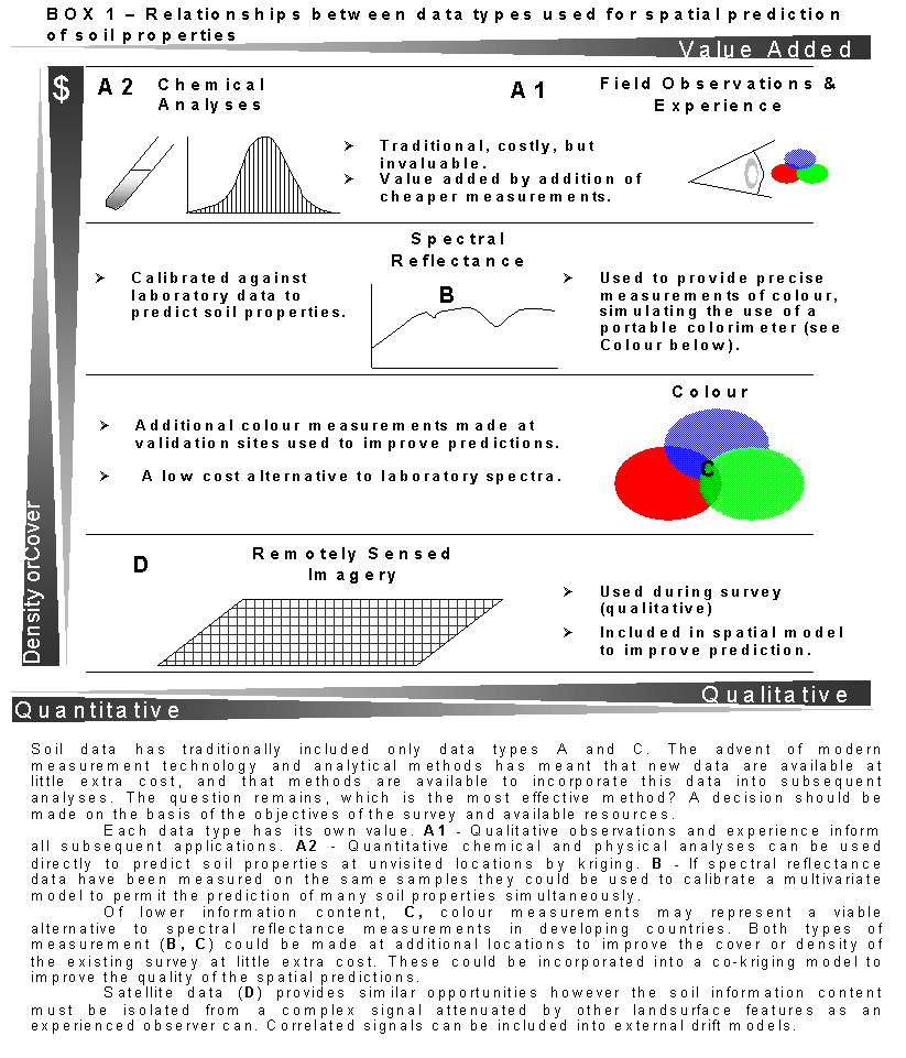
Efforts to provide cost-effective solutions to map the properties of the soil are the focus of this thesis. In the following chapters methods of measuring and predicting soil properties will be described and tested. Soil data has traditionally included only qualitative visual observations and expensive time-consuming chemical and physical analyses performed on samples transported to the laboratory. The advent of modern measurement technologies and analytical methods has meant that new data are available at little extra cost. Soil survey data can now commonly include traditional and modern data types for example,
- Qualitative observations of soil horizon attributes and soil colour
- Spectral reflectance measurements
- Optical and radar satellite imagery.
The cost of collection, the
information content and format of the data provided by each measurement method
differs significantly. Measurements made by
observation are invaluable to provide a first conceptual model of soil spatial
variability during the initial stages of soil survey. Physical and chemical
analyses are then necessary to validate the conceptual model and provide sample
averages for these properties for the region and by soil type. This is a
‘traditional’ approach to soil survey and the spatial prediction of soil
properties that suffers from several drawbacks:
·
visual observations are
subjective measurements and are poorly reproducible,
· soil survey and traditional laboratory analyses methods are time consuming and expensive,
·
traditional chemical and
physical analyses are destructive
·
the sample density and
coverage are limited by cost-time restraints,
Modern measurement technologies and statistical analyses offer a means of overcoming some of these problems. The most widely used of these technologies exploit the properties of electromagnetic (EM) radiation and its characteristic interactions with those of soil, permitting measurements of the quantities of reflected energy to be used as diagnostic of soil physical and chemical properties. The same characteristic interactions allow an observer to distinguish between soils. When colour matching the human eye is measuring the intensity of light energy arriving at the eye from distant objects, and then processing these stimuli with the brain. Observation is a ‘remote’ and ‘non-destructive’ measurement technique. Proximal sensing (PS) and remote sensing (RS) technologies also provide non-destructive measurements of distant objects by measuring the EM radiation coming from the object. Sensors are capable of measuring EM radiation with precision, over a much larger area and range of wavelengths than an observer can. But at present there is a three-way trade-off between these advantages (Figure 1. 1). The spectral, spatial and temporal resolution of different sensor systems are fixed system parameters that have to date limited the utility of ‘operationally’ available remotely sensed data. Exhaustive and large area spatial coverage landsurface measurements are available from satellite remote sensing devices such as the Landsat Thematic Mapper. But the poor spatial and spectral resolution of much of the commercially available optical remotely sensed data to date, are drawbacks that have implications for nearly all subsequent analyses.
The processes of isolating soil related information from such imagery are fraught with problems. Regardless of the precision of the sensor, vegetation often hides the soil completely in humid environments. While it is possible to interpret the presence or absence of a certain vegetation community with a given soil type it is not desirable to do so. The observations are not direct and there are no reasons why a given vegetation community should exist exclusively on a precise soil type. For this reason many of the applications of RS data to soil are restricted to arid and semi-arid environments (Escafadel et al. 1993), or to certain periods of the year when the soil is bare. Where the soil is entirely covered throughout the year remote sensing technologies provide only partial or surrogate information. Other concerns raised by the use of remotely sensed imagery include the possible error introduced by georectification and positional inaccuracies. Atmospheric absorption may hide important soil information carried by specific bands within these absorption regions. Poor temporal coverage may also render the data useless for the proposed purposes.
|
Figure
1. 1.
Schematic representation of the spatial-spectral-coverage trade-offs, when
measuring electromagnetic radiation at the Earths’
surface. |
Airborne hyperspectral data appears to offer a potential solution to many of these problems. Capable of being flown at any altitude they can provide high-resolution data that is only weakly affected by atmospheric absorption. Measurements can also be made with a temporal frequency dictated by the objectives of the study, or to collect data at specific times when the soil is bare. Still, the measurement provided by these sensors may not be ‘optimal’, because the sensors were simply not designed specifically for soil studies. Georectification problems can be exacerbated by the movements of the aircraft and the proximity of the scene. The spatial complexity of the images and the simple fact that there are so many individual measurements across many wavelengths may exacerbate the process of isolating soil related information from features of little interest, for example manmade features or simply shadow. There are very few studies that have successfully used remotely sensed data of any type to directly predict the value of continuous soil properties (Palacios-Orueta et al 1999). |

The use of RS data as soft ancillary information is more common (Odeh & McBratney, 2000). The majority of studies using such imagery use either classification or spectral un-mixing methods to provide abstract measures that relate to the landsurface as a whole, such as the percentage soil and vegetation cover or a degree of class similarity. The complexity of the landsurface and contamination of the soil reflectance signal by more dominant reflectors are such that remotely sensed imagery has perhaps been less useful than originally thought initially possible. When modelling at a coarse scale, soil parameter values identified from surrogate and often abstract information may suffice. However more detailed studies will require spatially distributed continuous parameters to drive soil processes. For this robust calibration and regression methods are required. All of these issues, which are discussed in greater detail throughout this thesis, suggest that the collection of ever-greater quantities of in-situ data cannot be avoided and is indeed necessary. A cheaper alternative to standard chemical and physical analyses is required. Spectral reflectance measurements made directly of the soil / landsurface or on samples in the laboratory offer this potential (Escafadel et al, 1993).
|
|
A compromise, which combines the cheap and rapid measurement processes offered by modern laboratory and remote sensor technologies with more standard chemical and physical analyses might represent the cost effective solution. Interpolation methods exist to spatialize the useful information derived from the spectral reflectance data measured at visited locations, using soft exhaustive data to improve the spatial estimates. Remotely sensed data is likely to have a greater correlation with data of a similar nature (electromagnetic) and this virtue should provide a basis for the interpretation of the relationships between the sensed signal and the soil in physical terms.
The progress in measurement technologies permits a flexibility that can provide solutions to certain of the issues raised above, but significant possibilities and questions remain to be explored and answered (see Box 1). The rest of this thesis is devoted to identifying solutions for the inclusion of measurements of the reflectance properties of the soil, into models for the prediction of soil properties.
Spectral reflectance measurements made on soil samples will effectively remove any confusing vegetation effects, but how should this multivariate data be used for soil property prediction; what are the alternatives to classification? What methods exist to reduce the dimensionality of this data while keeping the important soil information?
Data reduction is required for various reasons discussed later, not least, because the sensor systems where not specifically designed for soil studies and many of the measurements made may be redundant. Can the process of data reduction lead to the identification of simpler, cheaper measurements or representations of the soil that are better suited to soil studies or with which soil scientists are more familiar? How can the predictive potential of remotely sensed data be realised within this framework? What improvements in prediction quality can measurement technologies provide? Progressively four types of data including, qualitative observations of horizonation and colour, spectral reflectance measurements collected in the laboratory, colour measurements derived from these and remotely sensed data from operational satellites were explored for their information content and ability to predict soil properties. In the first two chapters standard methods were applied using traditional data types (A) to provide (non)-spatial predictions of soil properties. In the optimal situation of data availability explored in the final chapter laboratory spectral reflectance measurements and remotely sensed data augmented traditional chemical and physical analyses and observations made on samples collected in the field. The main body of this thesis involved the search for methods to overcome calibration problems posed by the high-dimensionality of the diffuse spectral reflectance measurements to enable their inclusion in (spatial) regression models. As well as testing multivariate calibration methods for hyperspectral data, methods were sought to reduce the dimensionality of reflectance data while retaining useful information content. Soil colour has always been an important diagnostic attribute and one of the most important characteristics used to differentiate soil in most systems of classification and soil survey (Stoner & Baumgardner 1980, Kingham 1998). The historical use of soil colour, as a diagnostic and predictive tool and its future role as a means of communicating reflectance information, are the theme of an entire chapter. Colour measurements were also tested as an alternative to hyperspectral data, reflecting a situation where the high-dimension spectrometer data is replaced by a low-dimension colour representation. Colour and remotely sensed data were also tested for their utility as a means to augment the amount of spatial information available and increase the precision of the final estimates.
In the rest of this first chapter the study area and traditional soil measurements, including qualitative soil observations and ‘standard’ destructive chemical and physical analyses are presented and the results of what could be considered ‘standard’ soil survey methods evaluated. While the end objectives of modern soil survey should inevitably lead to quantitative predictions of continuous soil properties the benefits to be gained from the process of observation and conceptualisation should not be disregarded as they indicate the correct framework and methodologies with which to take the analyses further.
The study area and survey data
Aridity was perhaps the most important criteria when identifying likely places to carry out this research. Soils under a low rainfall regime are less densely covered by vegetation, and therefore the remotely sensed signal is less contaminated by vegetation reflectance characteristics. A study site in southwest Niger, the focus of the Hapex-Sahel experiments (Prince et al. 1995) was the first location chosen for this reason and because of the abundance of freely available remotely sensed imagery. However it was not possible to complete the necessary fieldwork there.
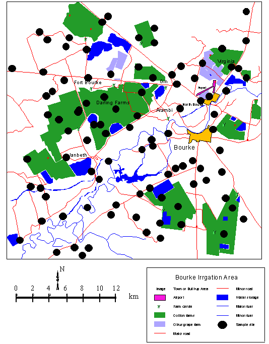
The fieldwork for the main body of this study was completed in southwest Australia. The Bourke region is approximately 700 km north-west of Sydney, New South Wales Australia. Bourke is located in the Eromanga Basin, a Jurassic to Cretaceous sedimentary basin that is part of the Great Artesian Basin of New South Wales. The Eromanga Basin is characterised by large expanses of low relief and extensive alluvial systems. The varied depositional environments of the Cainozoic era provided the sediments creating dunes and levées that have since undergone varied pedogenesis (Senior et al. 1978, Kingham 1998). The natural vegetation cover includes eucalyptus forest with a dense shrub understory or tall grass, which in many areas is extensively grazed by sheep. Cleared unimproved grassland extends onto the plains, which in recent years have seen the development of isolated agricultural enterprises. Cotton is the principle crop grown on the plains. In some areas citrus fruit and vineyards have been recently established.
|
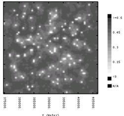
The soil survey that was completed during the Australian winter of 1999 covered an area of 900km2 and lasted one week. The number of samples collected and the density of the sampling scheme were designed to reflect a standard reconnaissance level soil survey. One hundred and fifty sample locations were selected using a stratified random sampling scheme (Figure 1. 2). Of the 150 locations chosen, 110 were visited and at each location at least one soil sample was collected. At each location visited a series of qualitative observations were made and recorded. These included vegetation structure (forest, scrub, grassland, crop) and moisture and erosion status and soil colour. At 20 locations a second sample was collected approximately 500m away from the first in a direction defined at random. Each sample was bulked from four smaller cores of the uppermost soil layer (0-10 cm) and collected over an area 20m by 20m. This area is approximately equivalent to the landsurface represented by a single Landsat image pixel. If the measurements have a similar support the correlations between them can be considered valid and is likely to be more significant. A total of 130 surface soil samples were collected of which 110 underwent a series of standard chemical and physical analyses (see Box 2, overpage). Iron content was measured by extraction in 1M hydrochoric acid extraction and organic matter / carbon by the Walkley Black method at a commercial laboratory. The acidity/alkalinity (pH) and electrical conductivity (ECe) were measured by electrode techniques in a 1:5 soil: deionised water solution. |
|
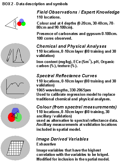
Soil texture was measured using the ‘micro-pippette method’, using only very small quantities of soil, (see Appendix for details). At 100 of the locations it was possible to drill soil cores to a depth of 1 m, from which the presence and thickness of diffuse and nodular carbonate horizons were identified using 0.1 M HCL. The solution was poured the length of the core and any effervescence noted. Gypsum accumulations, recognised as occupying greater than 10 % of the soil matrix, were identified using the method outlined by Verheye & Boyadgiev (1997).
Reliant on visual identification alone it is likely that in some cores accumulations were not observed where they actually existed. These techniques are not capable of identifying with great detail very thin horizons. There is a detection limit below which the horizon thickness has to be considered zero (~2-3cm). Horizon thickness data is a censored variable. From the same cores soil colour measurements were made of horizons are at four depths (0-20cm, 30-40cm, 70-80cm and 90-100cm) by comparing moistened soil with Munsell colour chips (colour matching). Details of the proximal and remotely sensed measurements and data are provided in subsequent chapters. The specific combinations of the various types of data used for each analysis as well as the validation methodology will be outlined in the methods description specific to each analysis.
|
Figure
1. 2.
Bourke Irrigation Area. Origin (bottom left): 37500 E,
6655000 N. |
MethodsThe rest of this introductory chapter describes the theoretical basis and application of ‘standard’ non-spatial and spatial regression methods for the characterisation and prediction of soil variability. The specific objectives were to 1. Describe and test the validity of a conceptual soil classification 2. Compare the basis of this classification with its quantitative counterpart 3. Provide estimates and maps of important soil properties 4. Investigate the spatial variability of the soil properties ClassificationTraditionally soil survey and the resulting stratification of the soil into more or less homogeneous units have been based solely on expert knowledge that informed an inductive logic. The framework most often adopted during the development of conceptual soil-landscape models, was developed by Jenny (1941). It states that the soil is a function of climate, parent material, topography, biota. Each of these conditioning factors varies more or less continuously over the surface of the Earth and so the properties of the soil vary in response. |
A conceptual model of soil spatial variability developed in the field is based on subjective interpretations of observations, and represents an informal rule based decision-making process. These models represent the first step in formalising the available knowledge about the soils of a region. Often the concepts underlying the model and the methodology required to allocate a soil using these concepts are hard to communicate to others. The model is personal to the soil surveyor. Diagnostic classification systems, for example Soil Taxonomy (Soil Survey Staff, 1975) formalise the rules of soil classification and standardise the description of soil variability, on the basis of the values of diagnostic soil properties. Formal systems are often criticised for being unwieldy, and providing an unrealistic hierarchical representation of soil variability (Webster, 1968). Considerable amounts of soil data, collected at all depths in the profile can be required to correctly allocate a soil to a class. Often this data is unavailable, and under such circumstances informal conceptual models or clustering methods must be adopted.
Quantitative methods of soil classification provide a robust alternative to conceptual models, a means of consistently and quantitatively describing the similarities and dissimilarities between samples using any number of variables that describe as many properties that can be measured (Oliver & Webster, 1990). Individuals can be represented in ‘n’-dimensional character space using various measures to describe the distance between individuals and groups (Gordon, 1987). Many iterative clustering algorithms exist to allocate samples to groups by seeking to minimise the within group dissimilarity of these measures.
Yet, by allocating samples to crisp groups numerical cluster analysis and formal diagnostic classification systems fail to represent the continuous nature of soil spatial variability. Conventional methods assign each location to a single group, regardless of the degree of similarity it shares with locations in other groups. They offer no means of representing the degree of (dis)similarity between two soils. The mathematics of fuzzy sets has provided some useful mathematical tools that correspond closely to our ‘human’ perception of difference (similarity). Zadeh (1965) is responsible for developing the concepts and mathematics behind fuzzy set theory that permits a continuous representation of the ‘degree of similarity’ between samples. Fuzzy classification (FC) methods are valued for their ability to express
a) generality – when a single concept applies to a variety of situations
b) ambiguity – a single concept embraces several subconcepts and,
c) vagueness – there are no precise boundaries
The FC algorithm minimises the objective function J(M, C),
where c is the number of classes, n is the number of samples, mij is the membership of an individual i in class j and d2 is a measure of dissimilarity (de Gruijter & McBratney, 1988). The main difference between Equation 1. 1 and a standard clustering objective function is the fuzziness exponent j (1 < j < µ). When crisp classifying the value of j is fixed at 1. For FC the value is usually fixed within the range 1.5 – 2.
Burrough et al. (1989, 1992) and McBratney et al.
(1992) originally applied fuzzy classification to soil data. It has since proved
popular because of its ability to represent soils within continuous character
space that reflects the spatial characteristics and our conceptual understanding
of how soils vary spatially. Burrough (1989) wrote that “too much flexibility
leads to anarchy and too much rigidity causes conflict.” Fuzzy set theory has
provided quantitative methods that enable the expression of both flexibility and
rigidity and the human concept of vagueness. Where conventional classifications
either exclude or include a soil from each class by associating class boundaries
with a membership cut-off value, a fuzzy classification describes the
relationship between a sample and all classes on a scale of zero to one
(zero = no similarity or shared characteristics). The FC algorithm has
since been modified (de Gruijter & Mc Bratney, 1988) to distinguish
modal soils, from soils that share properties with many groups (intergrades) and
those soils that bear no similarities to any of the class centroids
(extragrades).
Interpolation
Classification methods are useful when there are measurements of many soil attributes, and this information must be synthesised into a format, which facilitates its interpretation and communication. Increasingly, methods are required to predict the value of a single soil property at unvisited locations, instead of providing a more general description of what the soil is like everywhere.
The objective of soil mapping is to characterise this variability and to provide spatial predictions at unvisited locations. To do this a model of spatial variability is required. A general model of spatial variability of a soil attribute Z assumes some form of structural component m requiring a functional representation, and an error component e,
Equation 1. 2
![]() .
.
This model is very flexible. Traditionally the functional form of Z(x) was purely conceptual, difficult to communicate and irreproducible. In recent years mathematical and statistical methods have been applied to the problem and various quantitative models have been developed. They formalise a conceptual understanding of how soil varies spatially and provide a toolbox to characterise soil variability and provide predictions at unvisited locations.
During soil survey, empirical and conceptual soil-landscape models are developed to provide predictive information about the spatial distribution of soil classes Dk, over the study domain D. Laboratory analyses provide statistics that describe the average attribute values zk(x) for the class, k = 1 ,…, K present at each location x. The mean m(x), variance s(x) and prediction error e(x) are assumed to be constant within each class. This model is called the discrete (or categorical) model of spatial variation (Heuvelink, 1993) and it is often used to represent the results of a crisp classification. It is the format most often used with Geographical Information Systems, GIS (Burrough, 1989a) because it is simple to associate class statistics with maps in chloropleth or vectorised form. Yet, the assumptions that are made about the structure of the soil spatial variability are unrealistic; soil spatial variation is continuous (Webster, 1968). The categorical model of spatial variation is appropriate for the representation of discontinuous spatial variation, but is often adopted due to a lack of soil observations and sample data (Heuvelink, 1993). The way in which we represent the soil is a compromise between reality and the availability of data that provides useful and reliable information.
The traditional methods of extrapolation or ‘free survey’ that used observations of topography, vegetation and geology to delineate regions of homogeneous soils have largely been superseded by quantitative interpolation methods, for the same reason that quantitative methods now dominate the realm of classification. Tessellation, inverse distance measures, nearest neighbour interpolation, spline functions and trend surfaces have all been applied to the problem (Burrough, 1989). Each method has its drawbacks, for example, local interpolators use data inefficiently and global trend surface techniques fail to predict well at small scales. None of these methods uses the values of the data themselves to determine the spatial weighting and none can provide any measure of the estimation uncertainty (Webster & Oliver, 1990).
Geostatistics, the practical application of Regionalised Variable Theory (Matheron, 1965) developed as a response to these failings and has since evolved to provide a flexible toolbox of statistical methods to explore and predict the spatial, temporal and multivariate structure of data. The Theory of REV’s provides a continuous model of spatial representation. The data z at locations x made over a domain and describing a soil attribute are regionalised random variables z(x) which, within a probabilistic framework, are considered to be just one realisation of a random function Z(x). A random function is an infinite family of random variables at each location over the region of interest. Using the data values measured on sparse samples z(x), geostatistical modelling seeks to characterise the important parameters of the random function Z(x), the structural component of the model of soil spatial variability and e(x) the model error (Equation 1. 2).
The variogram
Geostatistics uses the variogram as a tool to describe the spatial pattern of an attribute and subsequently for prediction and simulation. The experimental variogram of a continuous variable, g*(h), is calculated as half the average squared difference between data pairs,
where N(h) is the number of data pairs within a given class of distance and direction. The experimental variogram is then modelled using an authorised variogram function (Journel & Huijbregts, 1978). The accuracy with which the variogram parameters are estimated, and hence the variable predicted, may be improved by the reduction of the influence of a small number of large values (Goovaerts, 1997). The spread of the sample histogram can be reduced by transforming the original z-data into normal score y-values,
where f is a normal score transform that relates the p-quantiles zp and yp of the two distributions (Rivoirard, 1994). The variogram of the y (xa) can then be recalculated using Equation 1. 3. Typically the y(xa) variogram model gY(h), has a smaller relative nugget effect and greater spatial continuity over short lag distances than its gZ(h) equivalent, because of the reduction of influence of extreme values.
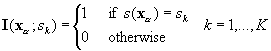
Indicator coding
Indicator variables,
I(xa ;zk), are generated by applying an
indicator transform to a continuous variable,
z(xa), at selected thresholds, zk which are
often chosen to be equal to the decile values of the cumulative
distribution,
Equation 1. 5
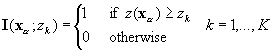
The indicator-transformed values describe the spatial
distribution of sets with random location and shape. Therefore the lateral
extent of a soil horizon can be described by a categorical indicator
variable defined at the threshold zk = 0. The
result is a categorical indicator variable equal to one if the horizon
sk, is present and zero if
not,
Equation 1. 6
The experimental variogram of an (categorical) indicator
variable I(x ; zk) is computed in
exactly the same way as that for continuous variables
as
Equation 1.
7
![]()
It describes the frequency with which two locations a vector, h, apart belong to different categories ¾ k = 1,…,K. This is also the probability of passing from one category to another for a given separation vector.
Ordinary and indicator kriging
Ordinary kriging (OK) and variants of this method are today the most commonly used interpolation methods to estimate the value of an attribute z at unsampled locations xa, using the surrounding n data {z(xa), a = 1,…n}. Kriging is optimal for the estimation of quasi-stationary continuous linear and additive variables from sparse sample data (Burgess & Webster, 1980a, b). Kriging systems are based on the same basic estimator Z*(x),
where la(x) is the weight assigned to the data z(xa) and m(xa) is the mean (Goovaerts, 1997). Simple kriging (SK) requires that the mean m (x) is known and constant across the entire domain to be estimated. For the majority of studies, this assumption is unrealistic. Ordinary kriging (OK) permits the relaxation of this constraining assumption of strict stationarity; the mean is considered constant only within a given local neighborhood W(x) of variable size surrounding the location to be estimated. For the estimate to be unbiased, from Equation 1. 8, it is evident that the spatial weights la should sum to one,
because this ensures that the mean error is equal to zero
Equation 1. 10 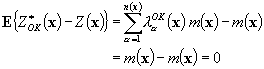
The
individual weights are then chosen so as to minimize the estimation variance
![]() , using the variogram to determine the spatial weighting
under constraint that the estimator is unbiased Equation 1. 9. The estimation variance is
, using the variogram to determine the spatial weighting
under constraint that the estimator is unbiased Equation 1. 9. The estimation variance is
Equation 1. 11 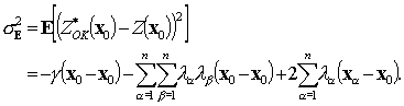
To minimise the estimation variance with the addition of the non-bias condition a zero sum expression including a Lagrangian L(u) parameter 2mOK is added to the equation for the estimation variance (Equation 1. 11). The ordinary kriging system (OK) is obtained by setting to zero the partial first derivatives with respect to each l and the Lagrange parameter
Equation 1. 12 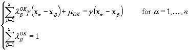
The estimation variance
equals,
Equation 1. 13 ![]()
The estimation variance is a measure
of the local uncertainty and is independent of the data values, that is, it
describes the estimation error at a single location irrespective of the
surrounding data and the value at the location
x0. It can be used to define the
optimal grid spacing (Webster & Oliver 1990) and a map of the estimation
variance is usually presented with each prediction. Thorough details and
properties of the ordinary kriging method can be found in textbooks by Goovaerts
(1997) and Wackernagel (1998). The series of papers by
Burgess & Webster (1980a-c) are a particularly good introduction
to the techniques applied to soil data. Bierkens and Burrough (1993) provide a
description of the indicator kriging system, which is discussed in greater
detail in the next chapter.
Geostatistical methods have flourished because of the flexible way in which models can be developed that are specific to the data that are being analysed. The constraint on the sum of the OK kriging weights is a good example of this. We cannot reasonably assume that the mean value is uniform across the domain neither do we have complete knowledge of the locally varying mean. The weight constraint incorporates this uncertainty into the model. So typically, for a given estimate the ordinary kriging estimation variance is larger than the simple kriging estimation variance. The choice of which system to use should be defined by expert knowledge of the data and the domain under investigation. The advantageous properties of kriging over other methods of interpolation include:
a) Efficient use of the data to define the spatial weighting and to predict.
b) Non-biased, exact estimates with minimum estimation variance.
c) Estimates can be made for isolated locations or areas of any size using a change of support model (Burgess & Webster 1980b).
d) Takes into account the sampling design and redundancy of information.
e) Local uncertainty is expressed through the kriging variance.
Kriging is used to provide optimal unbiased
estimates and a measure of the estimation error, not specifically to investigate
the uncertainty caused by the combination of spatial variability and incomplete
sampling. The predictions of soil properties across large regions from small
sparsely sampled datasets can be subject to considerable uncertainty, and a
study of this uncertainty may reveal as important as that of prediction itself.
Geostatistical simulation methods have been developed to generate many
equi-probable realisations (maps) of the RF, which have the same spatial
structure as the observed variable, regardless of the density or distribution of
the sample data. The spatial uncertainty information that they can provide
should represent a useful addition to the prediction and estimation variance
map.
Simulation
When sample data are sparsely distributed, the case for most reconnaissance soil surveys at a regional scale, considerable uncertainty is likely to be associated with each estimate. The estimation variance will be larger for samples that are more isolated, and for variables that have a large relative nugget variance. The rate with which the estimation variance increases with increasing distance from a sample location is determined by the structure of the variogram model (with the same range parameter). Clearly, the rate of increase will be slower when kriging using a Gaussian variogram that is continuous towards the origin, than when kriging using an exponential variogram.
The
kriging estimation variance and estimate of a multi-Gaussian variable can be
combined to provide conditional probability distributions ![]() that describe
the local uncertainty of the estimate at location x, using the
surrounding sample data, n. It is then possible to simulate local
uncertainty by drawing random numbers from this conditional distribution. But no
measure of the spatial uncertainty for a series of M locations can be
derived from the single-point ccdfs
that describe
the local uncertainty of the estimate at location x, using the
surrounding sample data, n. It is then possible to simulate local
uncertainty by drawing random numbers from this conditional distribution. But no
measure of the spatial uncertainty for a series of M locations can be
derived from the single-point ccdfs ![]() . Each estimate when considered individually is best (in the
least-squares sense), but the map of the local predictions “may not be best in a
wider sense” (Goovaerts, 1997). Most importantly, the estimation variance does
not describe the spatial uncertainty associated with possible patterns of
values.
. Each estimate when considered individually is best (in the
least-squares sense), but the map of the local predictions “may not be best in a
wider sense” (Goovaerts, 1997). Most importantly, the estimation variance does
not describe the spatial uncertainty associated with possible patterns of
values.
Simulation methods seek to reproduce global statistics such as the histogram or variogram in contrast to kriging, which seeks to optimise the local error variance (Goovaerts 2000). Simulation methods can be used to investigate spatial uncertainty with fine resolution from sparse samples. When simulating uncertainty information is provided by repeated computation of many equi-probable realisations. In contrast to kriging, simulation randomly selects a value z(x¢j), j = 1,…, N, at location x, from the N-point conditional cumulative distribution function (ccdf) that models the joint (hence spatial) uncertainty at the N locations surrounding the simulated point,
Eq. 1. 14
![]()
This process is repeated for each location x¢a, under constraints that include exactitude, global reproduction of the variogram and histogram of the random function. This does not mean that each individual realisation has the same histogram and variogram as the constraining data. Individually they can deviate considerably. However on average, if the realisations are considered together they should be reproduced. The individual realisations can also be analysed. Patterns that exist in many are considered likely to occur and those that appear irregularly rejected as improbable. The standard deviation can be calculated across all the realisations for each node to provide a measure of the spatial uncertainty prevalent at each node. A map of this variable could provide useful uncertainty information, for example, to identify regions of transition, where soil properties change rapidly and inversely those regions of homogeneous soil.
If the values at individual locations are the only focus of interest, simple kriging in a multiGaussian framework can provide similar uncertainty information. For local uncertainty investigation this is the perhaps the most efficient method, however with the speed today’s computers attain and the large storage devices that are available there is no reason why these techniques should not be superseded by simulation methods which can provide additional spatial uncertainty information that can be used in a number of ways. In contrast to kriged maps of continuous variables, thresholds can be applied to the realisations of a continuous variable because truncation of a single realisation of a random function generates a random set described by an indicator. The realisation sets can be used as inputs for further modelling activities to elucidate the effects of spatial uncertainty on the model outputs (Addiscott, 1993).
Many geostatistical methods exist to simulate both continuous and categorical (indicator) variables (Journel 1996, Goovaerts 1997). Turning Bands (TB), LU decomposition and sequential Gaussian simulation (sGs) methods can reconstruct the variability of realisations of continuous random functions. Sequential indicator simulation (sis) and truncated Gaussian (TG) methods are capable of generating realisations of random sets (Zhu & Journel, 1993). Both types of simulation method can be made conditional to sample data (Lantuéjoul, 1995). The methods can be further divided into two groups, sequential and non-sequential methods. A brief description of the concepts underlying the most commonly used sequential methods follows.
MultiGaussian Random Functions
The objective of simulation is to derive conditional
cumulative distribution functions (ccdfs) for each location. This is simplified
if all the ccdfs have the same analytical expression and are described by few
parameters, for example the mean and variance. To do so a model that describes
the complete multivariate distribution of the random function (RF) must be
assumed. The assumption of this model gives rise to the name parametric
simulation (Goovaerts, 1997). Combinations of variables
Xn, which have Gaussian statistical distributions
~N (0,1) have favourable properties of stability through addition
((X1 +
X2 = X3 is N (0,1)) and
through linear combination (lX1 + lX2 = X3 is N (0,1)), and
this can be generalised,
Equation 1. 15
![]() .
.
The central limit theorem infers that as ![]() , any combination of independent random variables
X1, X2,…, Xn, with zero mean and unit variance
has zero mean and unit variance,
, any combination of independent random variables
X1, X2,…, Xn, with zero mean and unit variance
has zero mean and unit variance,
Equation 1. 16 ![]()
Equation 1. 17 ![]() .
.
The variance of a combination of Gaussian
random variables remains constant if divided by the square root of
n,
Equation 1. 18 
Therefore it is possible to simulate
and combine many independent random variables each having the same mean and
variance as the original simulated Gaussian random variable ~N (0,Var(X)). The multiGaussian RF also
has favourable spatial properties. The two-point distribution of any pair of RVs
is normal and determined by the covariance function (Goovaerts, 1997). When
simulating to many locations the multiGaussian random function will have the
same variogram as the individual realisations if the variograms
g(h)i used to constrain the
selection of random values were the same.
Conditioning multiGaussian Random
Functions
Simple kriging lies at the heart of the majority of geostatistical simulation algorithms, because for multiGaussian random variables, the simple kriging error is uncorrelated with either the value of the estimated point or other estimated points, because the simulated values are linear combinations of the original independent random variables (Equation 1. 15). However the residual error is non-stationary, because SK is an exact interpolator. To simulate independent stationary residuals the following algorithm is used.
1)
Non-conditional simulation of RF,
Y(x) giving YS(x) at all
locations.
2)
Krige
using the YS(x) that coincide with data
locations as new samples to estimate a new variable
YS(x)K, which
satisfies,
Equation 1. 19 ![]()
3) Combine the simulated residual and an initial kriging estimate of Y(x), Y(x)K,
Equation 1. 20 ![]() ,
,
This process generates the normal simulated variable YSC(x) that is conditioned to the sample locations and variogram model, and honours the normal score transformed sample values at the sample locations.
The sGs method uses a moving window method and simulates points one after another, using already simulated values to update the neighbourhood and thereby contribute when simulating subsequent nodes. A simple overview of the process:
1) A random path across the domain is selected.
2) Krige the Yi(x) within a neighborhood surrounding a location, to give Y(x)K at all locations.
3) Simulate a variable ~N (0,1) and multiply this by sK, and add to either the conditioning data value or Y(x)K.
Simulating indicators
The basic idea behind the sequential indicator simulation algorithm is the use of indicator kriging to provide surrogate probabilities. Indicators for locations can be generated by drawing uniform values on a scale, U[0,1] and assigning either 1 or 0 depending upon the probability of occurrence p,
Equation 1. 21 ![]()
The probability of occurrence
depends on the values at surrounding locations. The conditional probability of
occurrence is equal to the kriged estimate of an indicator. Indicator based
simulation algorithms use the indicator kriging estimate as a conditional
probability (but one which can take values >1 and <0). If the indicator
function is considered as a random set
A,
Equation 1. 22 ![]() .
.
The value of the indicator of this
set known at the data points. The conditional probability of an indicator given
the surrounding data ![]() , then the simulated indicator is simply
, then the simulated indicator is simply ![]() . The most commonly used indicator simulation algorithm is
sequential indicator simulation (sis) Goovaerts (1997), that uses a random path
and a moving window method similar to the sGs method. Simulated values are used
to update the neighborhood information.
. The most commonly used indicator simulation algorithm is
sequential indicator simulation (sis) Goovaerts (1997), that uses a random path
and a moving window method similar to the sGs method. Simulated values are used
to update the neighborhood information.
The use of indicators methods to
provide posterior conditional probabilities can be criticized because the kriged
indicators are pseudo-probabilities that can exceed the [0,1] interval. Order
relation violations may also occur, when the cumulative probability at larger
quantiles is smaller than at lower quantiles. In practice the order relations
are usually solved by simply reordering and inadmissible values are typically
set to the maximum permissible values.
|
Figure
1. 3.
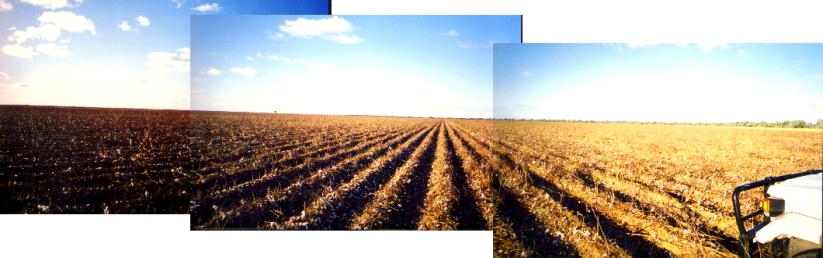
Cotton fields after harvest (June), showing the permanent ridge and furrow
planting scheme. |
|
|
|
Figure
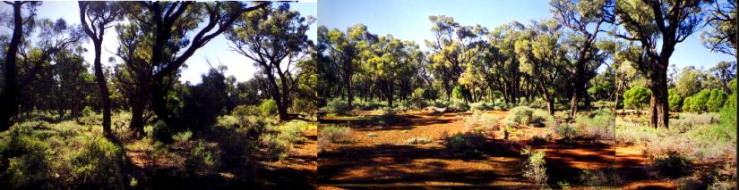
1. 4.
Natural eucalyptus woodland vegetation typical cover for the Red
soil |
Analyses and results
Conceptual classification, quantitative fuzzy classification and geostatistical interpolation/simulation, were applied using the ‘traditional data types’ (see box 1), which included visual observations of soil colour and chemical and physical analyses completed on 110 bulked samples of the upper 0-10cm soil layer collected in the field and transported to the laboratory. A total of 80 samples were used to calibrate the models while 30 were used for validation purposes.
Conceptual and quantitative fuzzy classification results were compared qualitatively to determine whether they represented a similar division of the samples. A quantitative comparison was not feasible because information about the profile properties of the soil unavoidably entered into the conceptual model. Only surface samples were included in the quantitative classification to permit comparison of prediction results with those from other methods presented later.
Kriging and simulation were used to provide estimate and spatial uncertainty maps of the continuous soil properties and the fuzzy classification memberships. These results were used to provide a preliminary indication of the precision that could be expected by applying current ‘operational’ techniques for soil mapping. Later they shall be compared with those provided by more elaborate methods, and when additional data is available at validation locations.
The conceptual model
Observations made in the field, interpreted in conjunction with the limited existing information for the region outlined earlier were the basis for a conceptual classification. The photographs on the subsequent pages summarise some of the observational information that provided the basis for this classification. Alluvial sediments in the low-lying plains have been transformed into grey (10 YR 5/2) clay soils, Vertosols (Isbell, 1996), used for irrigated cotton production and extensive grazing (Figure 1. 3, Figure 1. 6). Raised areas of higher relief (ancient dunes or levees) (~30 m) are covered by a mixture of fine- and coarse-sandy red or reddish (2.5 YR/V/C) soils, Rudosols (Isbell, 1996) which are thought to be of aeolian and fluvial origin (Northcote 1979). These soils are uncultivated, and support a natural forest vegetation (Figure 1. 4, Figure 1. 5). In the USDA (1975) classification these two soils would be allocated to the Vertisol and Ultisol classes respectively. These names are used interchangeably throughout the thesis.
|
Figure
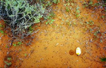
1. 5.
Typical Red soil surface, showing a small termite hole. Note the sandy
texture and intense red
colour. |
Figure
1. 6.
Cotton soil surface, showing cracking and accumulation of salts at the
surface, evidenced by the dominance of salt resistant scrub
plants. |
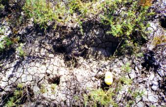
A light-coloured (5 YR/V/C), fine-textured ‘intergrade’ soil was observed on the slope breaks or the transition zones between the raised levees and low lying alluvial formation (Figure 1. 7). These transitional or intergrade soil for the region are described as Sodosols, Chromosols or Calcarosols in Isbell’s (1996) Australia Soil Classification, Alfisols in the USDA classification and Luvisols within the FAO system. Close to the present day river channel is a light-coloured fine silty coloured soil that has formed on the river levées. Gypsic horizons are found at depth in both Vertosols and Rudosols.
|
The A horizon of the Vertosols commonly have diffuse carbonates, while nodular carbonates are more common in the Rudosols. The sand, gypsum and the calcium carbonate are probably of similar aeolian origin. The region offers particular advantages for soil survey methods reliant on remote observations because of its semi-arid sparse natural vegetation cover. Also the land management practices associated with cotton farming leave the soil surface visible from space for long periods throughout the year. Each sample location was allocated while surveying to one of four soil classes; Cotton, Red, Levée or Transition classes, which correspond to the four soil types described above. Soil colour and texture were the key diagnostic attributes. Figure 1. 5 shows the distinct colour and sandy texture of the surface of a typical Red soil. |
Figure
1. 7.
A Transition soil surface, cracking like the Cotton soil, but with iron in
its oxidized form like the Red
soil. |
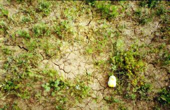
In contrast Figure 1. 6 shows the surface of a typical uncultivated Cotton soil. There is evidence of cracking caused by the shrink swell processes operating in this vertisol. The bright light colour is evidence of the build-up of salts at the surface. These two soil types can be considered as being modal for the region. The Cotton soil exists in the alluvial plains, the Red soil on the sandy dunes of an ancient landscape. The Cotton soil is homogeneous having uniform parent material, age and having undergone similar pedogenesis. The Red soil is more variable. The origins of the sandy dune materials is likely to have been more divers (aeolian and fluvial) and deposition is likely to have occurred during different periods over time.
|
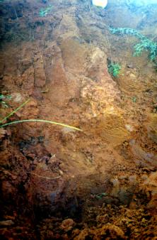
Figure
1. 8.
Red soil profile (showing depth of approx. 1.50 m), with duplex clay
horizon staring at 110 cm
depth. |
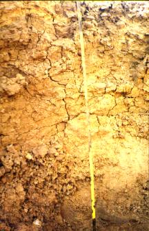
Figure
1. 9.
Well drained transition soil profile (showing depth of approx.
1.50 m), showing cracking in the upper
1 m. |
The Transition soil class is true to its name. Figure 1. 7 shows an example of the Transition soil surface. Its colour is ‘intermediate’ between the Red and Cotton soils and often samples allocated to this class were located along the boundary (or transition zone) between the two modal soil types. Relatively few samples of the Levee soil were collected. Samples allocated to this class were situated close to the present day river channel. In the conceptual model, these soils are young soils, with variable texture profiles that result from the heterogeneous depositional environment of the Murray-Darling River. Statistics for the laboratory analyses of chemical and physical analyses are presented in the appendix. The range of values observed for clay content are clearly in error. The cotton soils on the low-lying alluvial plains are vertisols. Hand texture analyses completed in the field indicated a clay content greater than 30% for these samples. The error was caused by the laboratory measurement method.
|
Figure
1. 10.
Box and whisker plots showing the distribution of values for the 0-10cm
sample for each soil type. (A = Levee, C = Cotton,
R = Red, T = Transition). The width of the boxes is
proportional to the number of samples allocated to each soil type, the
notch indicates the mean, horizontal bars +/- 2 standard deviations, and
the dots possible outliers. |
The processes of physical and chemical disaggregation did not successfully disperse and separate the clay particles from within larger aggregates. A more vigorous procedure should have been used to breakdown the strong aggregates caused by salinity and the presence of carbonates and probably gypsum. Nevertheless the remaining reliable chemical and physical laboratory analyses provided a means of validating the conceptual model and testing its predictive ability. Figure 1. 10 shows the statistical distribution of each measured variable for each soil type allocation. These plots show that the conceptual classification groups soils with similar properties. On average Cotton soils have larger silt, clay, organic matter, iron electrical conductivity and pH. The Red soil is sandier and has characteristically strong hue (intensity of colour) that distinguishes this soil from the dull grey Vertisol. Despite the strong colour of the Red soil, that would suggest intuitively that on average this soil has the larger iron content, it has less iron on average than the Cotton soil. The Red soil is sandier and the iron that is present coats the predominant large-grained sand particles and is therefore far more apparent. In contrast the Cotton soil is a vertisol with high clay content. It is regularly flooded, either as part of the on-farm flood and drain irrigation or when the Murray-Darling River breaks its banks. Iron oxides in the Cotton soil are reduced and intimately mixed with organic matter from the sediments contained in the river water, giving the soil a blue – grey colour. |
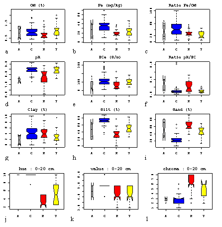
The transition soil forms an intergrade, with ‘intermediate’ sand and iron contents. On average cotton soils have higher organic matter content, pH and ECe than the red soil. These variables all show a wide dispersion of values about the soil type means. The results of a one-way ANOVA (Table 1. 1), using soil type to estimate the mean attribute value for each soil type confirmed that the conceptual model was capable of estimating the mean values of the pH, iron content, silt and sand content with a high degree of significance.Clay is poorly predicted because of measurement error. The distinction on the basis of soil type was less clear for electrical conductivity and organic matter content. They do not appear to affect the colour of the soil or reflect those properties that do in such a way that a human observer notices. On the other hand the sand and iron content contribute significantly to determining soil colour (Stoner et al. 1980), which is easily incorporated into a mental model of soil variability and was therefore diagnostic when allocating soils in the field.
Quantitative classification
During fuzzy classification the primary choice lies in determining the optimum number of classes (if the fuzzy membership coefficient is fixed). The conceptual model developed during sampling had four classes, two of which dominated the landscape, the Cotton and Red classes.
|
The Transition soil was identified as an intergrade and the Levée soil (poorly represented by the sample dataset) as resembling more the Cotton and Transition soil than the Red soil. Tests to define an appropriate fuzzy classification of the sample dataset indicated that only two classes could be adequately characterised. Figure 1. 11a plots the samples in the space of the first two transformed components of variation and from which two clear groupings are evident. Figure 1. 11b is a silhouette plot. |
Table
1. 1.
Summary of one-way ANOVA using soil type (L, C, R, T) to predict soil
properties. Level of significance: *0.1, **0.05, ***0.001. |
Each horizontal bar corresponds to one sample, the width of
the bar is calculated by
Equation 1. 23 ![]() ,
,
Where a(i) is the average dissimilarity between an individual and all other points of the cluster to which i belongs. Then for all clusters C, d2(i,C) is equal to the average dissimilarity of i to all observations of C. The smallest of these is denoted as b(i), and is interpreted as the dissimilarity between i and the cluster to which it has the second largest resemblance. The overall average silhouette width is the average of s(i) over all observations i and can be used to indicate the most suitable number of clusters. The larger the value the more reasonable is the choice of k. Figure 1. 11 shows two groups: the group to the right correspond to the Cotton soil, with 85 % of samples correctly assigned when in the field, the left hand group correspond to the Red soil (75 % same class). Several samples that bridge the gap formed by the two overlapping circles defining the fuzzy class boundaries (membership = 0). Another group of samples can be identified from the silhouette plot (Figure 1. 11b) having negative values of s(i). These samples bear little resemblance to either of the two classes.
|
Figure
1. 11.
Fuzzy classification of sample data (a) partition plot and (b) silhouette
plot. The symbols in (a) indicate the closest crisp allocation;
r
Red, ¡
Cotton. |
The former correspond to samples that were allocated to the Transition soil class, which can indeed be considered as an intergrade soil. The majority of the samples with negative s(i) values were allocated to the Levée soil group when in the field. Given that the fuzzy classification is generated using the sample data, the sample data should correlate with one or more of the fuzzy membership values. Unfortunately, the fuzzy memberships from the classification presented above were only very weakly correlated with the individual soil properties and regression was not feasible. |
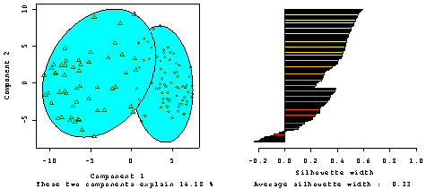
The total variance explained by the fuzzy classification is small (14.18%, see Figure 1. 11) because the division failed to account for the variance caused by the most statistically dispersed variables electrical conductivity and organic carbon content. Nevertheless, these results are testament to the validity of the initial subjective allocation to these classes and quantify the physical basis for the allocations. In-situ soil type allocation based on expert knowledge is a useful and cheap practice. The eye-brain combination is capable of adding considerable value to each sample observation and measurement and also isolating sources of noise that contribute little to the explanatory power of the model. The fuzzy classification mimicked this process quantitatively.
Interpolation and simulation
Structural analysis and interpolation
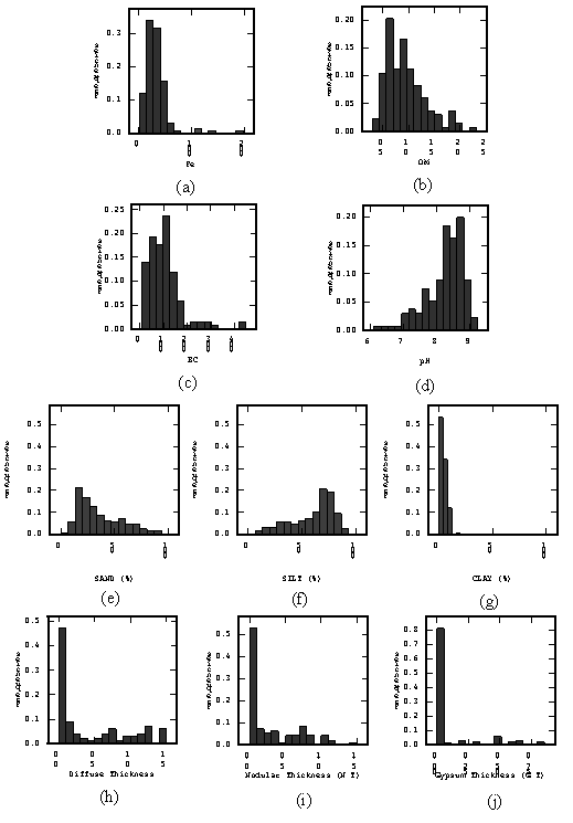
Histograms for each of the in-situ soil variables are presented in Figure 1. 12. They divide the data into two distinct groups. None of the variables has a distribution that could be described as normal, but the variables describing horizon thicknesses (Figure 1. 12h-j) are very positively skewed. The ordinary kriging estimator makes no assumptions about the shape of a variables statistical distribution, but OK estimates may suffer from exaggerated systematic bias caused by skew (Saito & Goovaerts, 2002). The positive skew of the horizon thickness variables is caused by the discontinuous spatial cover of the horizon attribute. A detailed analysis of these ‘discontinuous’ horizon attributes was completed separately so that various kriging methods could be tested and an appropriate method selected. The results of this analysis are presented in chapter 2. For the other variables, variograms were calculated in four directions with a lag spacing of, 2500m for 8 lag distance using the entire dataset (Figure 1. 13).
|
Table
1. 2.
Variogram models of soil properties of the Bourke region. For an example
of the notation, Stable (2) refers to a stable model with shape parameter
with value 2 |
When kriging the dataset was divided into training and validation sets, however the small size of the dataset meant that no samples could be set aside for variogram analysis, without introducing concerns about variogram stability. Predictions are always subject to uncertainty, because of approximations in the model, and error in the measured values the model parameters and variables. Variogram estimation requires at least 100 data points (Webster & Oliver, 1992). Estimating the variogram using just the validation points would have introduced an extra source of error that risked hiding the effects of the estimator on the quality of the predictions. | ||||||||||||||||||||||||||||||||||||||||||||||||||||||||||||||||||||||||||||||||||||||||||
|
The experimental variograms for each variable showed no evidence of geometric or zonal anisotropy, but all were erratic so a single non-directional variogram was modelled for each variable (Figure 1. 13). The fitted models fell into one of two groups. The first included the attributes pH, ECe and clay content, which have one short-range structure that does not exceed 5000 m and a large relative nugget effect (in particular clay content because of measurement error Figure 1. 13g). The range of the structural component of the second group, which included iron and organic carbon content, and (fuzzy) class membership was of the range 8000 – 10000 m. These parametizations suggest that short-range processes operating across the landscape are responsible for the chemical properties of the soil, and that these are in turn related to the clay content of the soil. This makes physical sense, because clay is the chemically active component of the solid soil fraction which controls to a large extent the pH buffering and salinity status of the soil. However this interpretation must be considered
carefully given the measurement error of the clay content data. Sand and
iron content appear to vary across larger spatial scales that reflect the
geomorphological characteristics of the region, the alluvial plains and
raised dunes. They share the same spatial characteristics as the regional
soil classification. Each of the raw variables was transformed into a zero mean Gaussian variable with unit variance for the purposes of simulation. Authorized models were fitted to each of these variables normal score experimental variograms. The models closely resembled those of the corresponding raw variables but as expected having lower nugget variance. |
Figure 1. 12. Histograms of soil chemical properties: (a) pH, (b) ECe (Sm-1), (c) organic matter (%), (d) Fe (mg / kg) (e) sand, (f) silt and (g) clay content, (h) diffuse, (i) nodular and (j) gypsum horizon thickness. |
|
Figure
1. 13.
Variograms of soil chemical properties: (a) pH, (b) ECe
(Sm 1), (c + g) organic matter (%), (d) Fe
(mg / kg) (e) sand, (f) silt and clay (g) content
(units = %), (h) fuzzy class members 1 and 2 (which have
identical variograms). |
The variogram models of the raw variables were used to predict each in-situ variable to the set of validation points. The same models were used to krige the prediction and estimation variance maps, using the entire dataset. The validation dataset was used to calculate the mean square error and the correlation between the true and predicted values, both measures of the quality of the fit. Kriging was performed in a moving neighbourhood that was large enough to ensure that all points in the domain could be estimated. The variograms of the normal score transforms of the soil variables were then used to simulate using sequential Gaussian algorithm (sGs). Tests were completed to identify the minimum number of simulations acceptable (50 to 5,000). The test results changed
little above 100 realisations. One hundred simulations of each variable
were generated and the results post-processed to calculate the simulation
standard deviation. Various parametizations of the moving window were
tested. Finally only a maximum of five simulated data values were included
in each window. The
quality of the OK estimates were evaluated using the validation statistics
(Table
1. 3) calculated at the 30 validation sample
locations. The root mean square error is expressed both in the original
units, but also as a percentage of the average value of the sample data.
The correlation value measures the degree of systematic prediction bias,
caused by the overestimation of low values and underestimation of high
values. The sparse nature of the dataset inevitably meant that the prediction quality would leave much to be desired. In the absence of many constraining data the predicted values tended towards the mean value. The most accurate and least biased predictions were for sand, silt and iron content and pH, the worst for organic carbon, ECe, and clay content. Again the quality of the latter is the poorest, further proof of measurement error, if needed. Table
1. 3.
Validation dataset prediction mean square error and correlation statistic
between true and predicted values. % error = rmse /
variance |

|
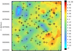
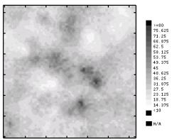
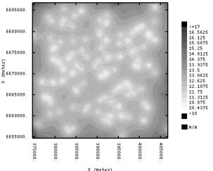
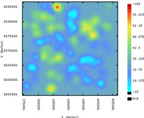
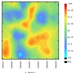
Prediction maps for each variable are
presented in Figure
1. 14 through figure 1.17. As the variogram
models indicated the prediction maps were to fall into two groups, a
function of the range of the fitted variogram model. The poorly predicted
variables ECe and organic carbon (OC) had short-range variograms
(~4000 m). Their prediction maps failed to reveal a strong
regionalisation. In contrast the prediction maps of iron content, pH,
texture and fuzzy class memberships, modeled using longer range variogram
structures (8000 – 10000 m), show a clear regional scale
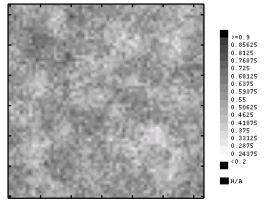
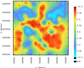
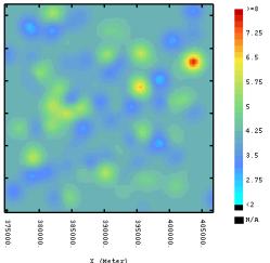
spatial structure. The density of the sampling is sufficient to characterize the regional scale variability of these attributes. The fuzzy class membership predictions show three regions with high Red soil memberships (ultisols-alfisols) corresponding to the southwest-northeast sandy dunes and ancient fluvial levees. (member 1, figure 1.15c d). A sinuous swath of vertisols soils (member 2) traverses the study region. The prediction maps for sand and silt content (figure 1.17a and b) resemble the fuzzy class membership maps. The clay content maps must be evaluated with caution because of measurement error. The sand and silt maps provide a clear indication of a swath of soils with high silt content (and consequently high clay content), corresponding to the high class 2 membership predictions. |
(a)
(b)
(c)
(d)
(e)
(f) Figure
1. 14.
Ordinary kriged (OK) map (left column) and sequential gaussian simulation
set (n = 500) standard deviation (right column), for pH
(a + b), ECe (c + d), organic matter
(e + f). |

|
(a)
(b)
(c)
(d)
(e)
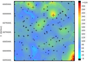
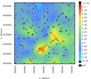
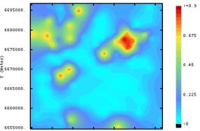
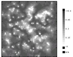
(f) Figure
1. 15.
Ordinary kriged (OK) map (left side) and sequential Gaussian simulation
set (n = 500) standard deviation (right side) for iron content
(a + b) respectively for Red soil member 1
(c + d) and Cotton soil member 2
(e + f). |
This sinuous feature describes the location of
depressions where fines have accumulated and where vertisols have
formed. Estimation variance maps for the best and
worst predicted variables are illustrated in Figure
1. 16. The estimation variance map provided no more
information other than that which is evident from a straightforward
diagram showing the sample locations combined with a knowledge of the
variogram model. Absolutely no difference can be observed between the two
maps. They
are an indication of sample density and as previously discussed the choice
of variogram, its parametization and the sample design, but provide no
variable specific uncertainty information, only model specific uncertainty
information.In contrast the simulation maps for each variable differ
considerably and can be interpreted very intuitively. The maps indicate
the regions where uncertainty is prevalent, caused by the heterogeneity of
sample values. The
uncertainty values are independent of the sample location distribution or
density. The patterns of values at the constraining sample locations
determine the structure of the variable specific spatial
uncertainty. |
|
(a)
(b) Figure
1. 16.
Maps of the OK estimation standard error for (a)
Fe* OK and (b) pH*OK,
illustrating the inutility of expressing variable specific spatial
uncertainty using the estimation variance, when the sample locations are
sparse and irregularly spaced. |
The simulation standard deviation maps of
the fuzzy class memberships show how region is dominated by vertisols
(member 2). The high degree of certainty of the presence of this soil is
illustrated by the uniformly low simulation standard deviation values
(figure1.15f), with spatially uniform the cotton
soils. This finding, suggests that cotton
production could be extended to similar regions with a strong likelihood
of finding similar soils. |
|
Figure
1. 17.
Ordinary kriged (OK) map for (a) sand (b) silt and (c) clay
content. | |
|
In
contrast the spatially heterogeneous and localized nature of the Red soils
was apparent from figure 1.15d. This map shows only two isolated
regions to the northeast of the region where member 1 (red soil)
uncertainty is low. Figure 1.15e and f show low values of
uncertainty to the center of the study area corresponding to the center of
the region dominated by the Cotton soil. In
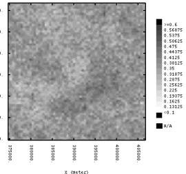
Figure
1. 14a c d the simulation standard
deviation maps reveal a heterogeneous short-range structure. This
indicates that the sampling strategy is insufficiently dense to capture
much of the spatial variability of these properties. The reasons for the
variability are not regional, but field scale and related to land
management practices and landcover type. Indeed, these soil properties are
likely to be significantly modified by very local activities and soil
processes, in particular the waterlogging, flooding and draining on the
cotton fields or local salinisation close to raised water storage
tanks. | |


Conclusions
The purpose of this first chapter was to
provide an introduction to the study area and to investigate the data. A
reminder of the first two objectives outlined earlier
:-
1. Describe and test the validity of a conceptual soil classification
2. Compare the basis of this classification with its quantitative counterpart
A considerable amount of information and data was gathered during just a single week of soil survey. The process of visiting all of the sample locations, augering and recording observations of the soil proved very informative. It became evident that three soil types dominate the landsurface; large homogeneous vertisol plains, raised dunes with less unfertile ultisols with large tracts of more fertile alfisols forming the transition between them. Ranges of soil physical and chemical properties strongly reflected this division, when not contaminated by measurement error. Unfortunately the clay content values could not be trusted. The conceptual classification of Red, Cotton and Transition soils is by no means a formal one, but it serves its purpose. It is a shorthand means of communicating that which has been learnt during the survey. As more data is collected and information synthesised about the soils of the study area, these expressions can be replaced by more detailed and precise allocations within formal systems. Importantly though, these results confirm that experience and observation can combine to permit the development of empirical and conceptual soil classification models, which have a predictive capability for those soil properties that clearly distinguish the soils of a region.
Lacking sufficient data to allocate each
sample accurately to a formal classification system, it was very important to
validate the underlying concepts of this rough and ready model using a
quantitative technique. Fuzzy classification methods
permitted the quantification of a conceptual model. The results of this
classification strongly reflected the original division of soils made in the
field. The same variables were diagnostic for both the
conceptual and quantitative models. Both models distinguished between soil types
primarily on the basis of their colour, their iron and sand content. Colour was
the main diagnostic soil property, because the relative proportions of sand and
iron content play a large role in determining it.
The next objectives were to:
1. provide estimates and maps of important soil properties and
2. investigate the spatial variability of the soil properties.
The results of any soil classification must
be transferred to a spatial representation to fulfil their predictive role.
Ordinary kriged estimates represent the ‘control’ in this study against which
the relative merits of other methods will be evaluated. Crisp soil
classifications stratify the landscape into uniform homogeneous regions. As
discussed, this representation contrasts with our understanding of the soil as a
continuous phenomenon, but could represent an acceptable level of
simplification, depending upon the scale of the soil survey. That which may be
perceived as continuous change at one scale of observation, could accurately be
represented at a lower resolution as a discontinuity without much loss of
generality. However, experience has shown that when a crisp classification is
transposed into the landscape the spatial representation is fragmented and bears
little resemblance to that which we intuitively know to be correct. By reducing
the fragmentation in character space caused by inappropriate exclusion from a
given class, spatial contiguity in the spatialisation of a classification can be
generated (McBratney et al. 1992).
The fuzzy classification membership maps
clearly show the expanses of Red soils, formed on dunes to the north-east and
west, also the isolated occurrence of a not dissimilar soil to the center west
of the study area. The large homogeneous expanse of Cotton soil, almost
exclusively exploited for cotton production, is identified as running in a swath
from the northwest to the southeast. This zone lies perpendicular to the present
course of the Murray-Darling River, whose presence is indicated by a thin swath
of low membership 2 values passing from the northeast to the
southwest.
Mapping the continuous fuzzy class memberships
has provided a quantitative method to mimic the minds ability to express the
vague human concepts that underlie conceptual models of soil spatial
variability. The procedure of combining the many univariate measurements into a
multivariate representation has isolated the regional components of spatial
variation. The process has filtered out the numerical fluctuations associated
with the variables that describe the individual soil attributes, and provided a
continuous numerical representation of their communality. As a result, the maps
of the kriged the fuzzy class memberships were less affected by individual
sample variation that are the exception, but by the features common to all
samples, global features of the dataset.
Finally,
simulation provided a useful alternative to the estimation variance map; the
simulation standard deviation maps provided spatial information that was a)
specific to each variable, b) a function of the chosen variogram model and, c)
the relative spatial distribution of the values. These maps permitted the
identification of regions where the value of the attribute could be expected to
be relatively constant, and the contrasting transition zones of rapid change and
spatial heterogeneity. Where spatial uncertainty was greatest more samples are
required to provide a uniform prediction quality. The value of the simulation
standard deviation could be used to choose the location of these
samples.
If anything this chapter has shown how pedological
observations can provide very useful spatial information at little cost. It
remains to explore the information content of the horizon observations that were
not included in the fuzzy classification of surface samples. Preliminary
investigations of this data suggested that alternative methods would be required
to provide accurate spatial predictions. The next chapter addresses these issues
in further detail.
Chapter 2
Predicting and simulating the
geometry of
soil horizons
Introduction
Pedological observations have traditionally formed the
bedrock of soil survey and shall continue to do so as long as resources are
scarce or until sufficiently precise and versatile, cost effective technological
alternatives are developed. During the reconnaissance stage of soil survey the
focus of attention has to be on providing an overview with which to create the
framework to describe and further investigate the soil spatial variability.
Pedological observations are essential to provide important ancillary (spatial)
information for inclusion within the conceptual model. When cost constraints
limit the use of detailed analyses to the upper layers of the soil observational
measurements may be the only way to provide a first overview of the profile
properties of the soil. They may also provide information invaluable in its own
right. Soil variation has long been described with reference to diagnostic
horizons, the presence or absence of which determines the allocation to a given
soil type in formal classification systems. Within the horizon the soil
properties (concentrations, density etc) are assumed to be uniform. This
represents a reasonable approximation for studies at coarser scales, typical of
GIS , regional or global studies if care is taken to accurately represent the
aerial and vertical extent of the horizon correctly.
Concerns about global climate change require estimates of various components of atmospheric and terrestrial carbon. This is particularly important with respect to terrestrial inorganic carbon, which is a major repository of global carbon dioxide (CO2). Global and regional estimates of inorganic carbon, particularly soil carbonates are particularly unreliable and in many cases do not take into account the spatial variability of the occurrence or the amount of carbonates in the soil horizons or examine the spatial variability of the predictions. Gypsum on the other hand is important for soil management. Worldwide estimates of the extent of soils containing gypsum range from 90 million (FAO, 1993) to 207 million ha (Eswaran and Zi-Tong, 1991). These estimates are as unreliable as those of terrestrial carbonates. There is, therefore, the need to design appropriate approaches to provide an inventory of soil carbonate and gypsum, particularly at the regional level, which could be aggregated to give estimates at the national, continental and global scale. Of specific concern in the Bourke region are the possible effects that carbonates and gypsum may have on soil stability with the introduction of irrigation.
It is increasingly important to provide uncertainty information concerning these predictions that can be propagated through soil, crop and climate models (Addiscott, 1993). Uncertainty arises in any situation where there is a lack of complete knowledge. Spatial prediction uncertainty is caused both by a lack of precision when collecting data and incomplete knowledge, an unavoidable characteristic of data provided by any measurement process and particularly prevalent when the data is collected across a large area from few sparsely distributed point samples.
Accurate spatial prediction of soil horizon thickness
implicitly requires accurate prediction of the locations where a horizon is
present. Soil horizon thickness can be expected to lie within a limited range of
values, whereas the true horizon lateral extent can differ considerably from
that indicated by the samples collected only at a few points across a region.
Therefore the uncertainty associated with the prediction of the horizons lateral
extent is likely to be far greater than that of predicted horizon thickness.
Geostatistical interpolation and simulation techniques can be used to provide
spatially distributed predictions and uncertainty measures, but the choice of
which technique to use should be defined by our understanding of the pedology of
the region and the data themselves. For example, ordinary kriging alone, may not
be the most suitable technique to estimate soil properties that are not
spatially continuous across the region, at the scale of observation, and hence
require a prior delineation of the zones within which the property can be
reasonably considered to be continuous (Voltz & Webster,
1990).
Soil
horizon thickness is a continuous variable often having a positively skewed
distribution. This is caused by many zero values, where no soil horizon is
present, and few extreme values. Ordinary kriging (OK) predictions of positively
skewed data are often biased, caused by the underestimation of large values and
overestimation of small values. Several geostatistical techniques have been
developed to overcome the prediction bias caused by positive skew, these include
multi-Gaussian kriging (MG) and indicator kriging (IK). A third method consists
of using the kriged prediction of an indicator of horizon presence to delineate
regions where the soil horizon is most likely to exist, and which can be used to
mask the continuous estimate. Zero values of the continuous variable delineate
the region where no horizon is present.
At a
regional scale of mapping and typically within GIS the boundary between regions
of horizon presence and absence are as discontinuities. The prediction of local
soil horizon thickness could consist of an initial prediction of the regions
where the soil horizon is present, and within which it can reasonably assumed to
be continuously spatially distributed, followed by an optimal estimation of the
continuous variable within these zones. In some respects this is a similar
approach to that suggested by Voltz & Webster (1990), the main
difference being that the data themselves are used to delineate the regions of
horizon presence and absence instead of a pre-existing soil map. The benefits in
terms of prior data requirements are evident, in particular for regions where no
prior observations or map delineations exist.
Any
statistical prediction is subject to uncertainty (Journel, 1989), but this is
exaggerated when the number of samples is small and the distance between samples
large; a feature typical of regional scale reconnaissance soil surveys. By
recreating sample variability simulation techniques can provide information
describing the spatial uncertainty of the attributes across the study area
additional to the local measures provided by kriging, such as the estimation
variance. Again, there are many geostatistical algorithms available to simulate
both continuous and categorical variables and the results that they provide can
differ (Journel & Isaaks 1984, Goovaerts, 2001).
In this chapter, methods to estimate soil horizon attributes thickness and lateral extent using a simulated dataset that shared the same statistical and spatial properties exhibited by a real dataset were compared. The objectives were: (i) to apply the method that performed best to the real in-situ data and (ii) then to investigate the uncertainty associated with the prediction of the soil horizons lateral and vertical extent by geostatistical simulation.
Kriging continuous attributes with positive
skew
The
ordinary kriging (OK) system is derived under the assumption that the mean
m(xa) is constant but unknown within a local neighbourhood
W(x). Therefore the local mean must be estimated for each
z(xa). This estimate is not robust to the presence of extreme
values. Systematic prediction bias can be severe for positively skewed data. A
single extreme value can impact the estimate of the local mean and cause under
and overestimation of the tails of the z(x) histogram. This is
known as the ‘smoothing effect’. Smoothing increases with increasing skew,
relative nugget effect and with decreasing sample density (Goovaerts,
1997).
Techniques have been developed to reduce systematic
prediction bias caused by skew, namely multi-Gaussian kriging (MG) and indicator
kriging (IK). Both require a non-linear (back) transform of the data prior
to and after kriging. The first step of multi-Gaussian kriging is the
normalisation of the z(xa) to generate a variable with a Gaussian distribution. This
facilitates inference of the mean when kriging. The kriging estimates
Y*SK (xa) are then back-transformed to provide the estimate
Z*MG(x).
Indicator kriging involves variogram modelling and kriging
for the suite of indicators defined using equation 1. The prediction
Z*IK(x) is obtained by multiplying the
estimate at each threshold zk by the threshold value
and summing the results for all K. Nevertheless, because kriging is a
form of weighted spatial averaging OK, MG and IK can all be expected to produce
a smoothing effect of the true Z(x) histogram. When kriging the
high-frequency short-range variability represented by the nugget effect is
filtered. Extreme and erratic values are not generated other than at data
points. As the sample density decreases and the predictions tend toward the mean
value the smoothing effect can be expected to increase. Therefore none of these
interpolation methods can be used to classify zero and non-zero zones based on
the predicted values. Indeed if any cut-off is applied to the kriged estimate to
provide an estimate of the areal cover of the horizon it too will be biased.
Instead an estimate of the probability of the threshold value occurring is
required.
Kriging categorical attributes to delineate zones of
presence
Consider a categorical indicator defined on the basis of
presence or absence. The sample mean of the indicator is a prior estimate of the
probability of the category’s presence. The kriged estimate of the categorical
indicator represents its conditional expectation, which in turn equals the
conditional probability that the category sk is
present,
Equation 2. 1
![]()
where |n stands represents
the conditioning of the prediction by the surrounding n data surrounding
a location x. Because the estimate is can be interpreted as a probability
it is possible to threshold and thereby to indicator code the kriged
estimate,
Equation 2. 2
The resulting indicator variable delineates the most probable zones of horizon presence and absence. In the absence of prediction bias a reasonable classification criterion would ensure that the estimated lateral extent should equal the global sample proportion. For an unbiased estimate, values smaller than 0.5 indicate a greater likelihood of absence than presence and vice-versa. If available other sources of information could be used to inform this choice, or thresholds can be applied at various values to provide an indication of the uncertainty of the predicted aerial extent.
Methods and Analyses
A
sensible approach to the estimation of local horizon thickness should involve
two-steps; an initial delineation of the zones where a horizon is most likely to
be present and an optimal kriging of horizon thickness within these zones. This
hypothesis was tested using a simulated dataset because the in-situ
dataset consisted of relatively few sparsely located samples (100 auger
observations). Under such circumstances the comparison of prediction methods on
synthetic data with similar statistical properties as the real data represented
a useful alternative to cross-validation, for hypothesis testing and
investigating uncertainty caused by the choice of technique. The construction of
a simulated dataset necessarily started with a detailed analysis of the true
sample data to ensure that the simulated data had similar statistical and
spatial properties.
The second part of the analysis involved a comparison of the tools that were available to provide information describing spatial uncertainty. In the first instance the measures provided by kriging and simulation methods were evaluated and compared. Finally the difference between the measures of uncertainty of horizon lateral extent provided by parametric sGs and non-parametric sis algorithms are discussed.
Structural analyses of horizon attributes
The in-situ variables used were presence (or absence) of: 1) diffuse CO32+ (D), 2) nodular CO32+ (N) and 3) gypsum (G). We refer to the categorical indicator variables as I(x ; D) for the diffuse CO32+, I(x ; N) for the nodular CO32+ and I(x ; G) for gypsum. The horizon thickness values are DT, or NT, or GT, respectively, with subscript T indicating the thickness. The sample data indicate that, the diffuse carbonate horizon is more prevalent than horizons with carbonate nodules.
|
Gypsum horizons are relatively uncommon, being present at only 20 % of the sites. However, the lack of an explicitly defined test method and the reliance solely on visual recognition of its presence as crystals coatings found within the profile probably led to an underestimation of gypsum. The mean depths of the upper depth limits followed the expected
pattern with diffuse carbonates typically occurring closer to the surface
than nodular carbonates, and the latter forming above gypsum
concretions |
Table 2. 1. Variogram parameters of in-situ horizon indicators (D, N, G), the normal score transforms of in-situ horizon thickness (DTg, NTg, GTg) and the simulated transect thickness TSIM and lateral extent PSIM (discussed later). | ||||||||||||||||||||||||||||||||||||||||||||||||||||||||||||||||||
|
The diffuse carbonate horizon often extends into the nodular carbonate horizon as expected. The correlation between indicators suggests that nodular calcium is often co-located with diffuse carbonates (r = 0.45). Their spatial co-dependence is weak and intrinsic. Gypsum shows a very weak negative intrinsic correlation with diffuse and nodular carbonates (r = - 0.09). Intrinsic spatial correlation occurs when the properties have the same basic variogram structure and proportional sill variance. Variogram models of the thickness variables for each horizon are shown in Table 2. 1 and Figure 2. 1. Each was modelled using a combination of a nugget effect and an exponential model. The nugget effect accounted for over half of the modelled semivariance for each horizon type, being largest for the nodular horizon and smallest for the diffuse carbonate horizon. Gypsum and diffuse carbonate horizon exponential models had a similar long range (15300 m and 24280 m respectively), in contrast to that of nodular carbonates, which was approximately half this distance. For the purposes of multi-Gaussian kriging and
simulation, each thickness variable was normal score transformed and the
variogram fitting procedure repeated. The resulting models all had smaller
relative nugget effect and greater spatial continuity as evidenced by the
longer range of the fitted exponential odels. |
Figure
2. 1.
Experimental (dots) and modelled (thick line) variograms for (a) diffuse
carbonate indicator, (b) diffuse carbonate thickness, (c) diffuse
carbonate thickness normal scores, (d) nodular carbonate indicator, (e)
nodular carbonate thickness, (f) nodular carbonate thickness normal
scores, (g) gypsum indicator, (h) gypsum thickness, (i) gypsum thickness
normal scores.
Simulating a dataset
with realistic characteristics. | ||||||||||||||||||||||||||||||||||||||||||||||||||||||||||||||||||
|
Variograms were also fitted to the (categorical) indicator variables of each horizon. Again each was modelled using a combination of a nugget effect and exponential model. Interestingly the exponential model ranges of both diffuse and gypsum indicators were approximately half the length of the corresponding thickness variables, while that of the nodular carbonate indicator was twice the length of its thickness counterpart. This suggests that nodular carbonates are widespread but extend to very different depths over short distances. In contrast diffuse carbonates and gypsum are localised and dispersed. For each variable, the variograms of indicators defined at increasingly large decile values showed a typical destructuration effect (Figure 2. 2). For a cut-off greater than 1 m the models were almost pure nugget effect. Thirty values were drawn at
random from a Gaussian distribution N (0, 1) at equidistant locations along a
hypothetical 25 km long transect. The variogram model Figure
2. 2.
Indicator variograms for selected cut-offs applied to diffuse horizon
thickness, zk (a) z1 = 0.06 (b)
z2 = 0.15 (c) z3 = 0.32 (d)
z4 = 0.51 (e) z5 = 0.67 (f)
z6 = 0.83 (g) z7 = 1.13 (h)
z8 = 1.27 (i)
z9 = 1.36.
(REMOVED) Finally a categorical indicator was defined to create
the simulated horizon lateral extent PSIM, | |||||||||||||||||||||||||||||||||||||||||||||||||||||||||||||||||||

and a
variogram model, ![]() , was adjusted to this variable to be used for kriging the
indicator of presence / absence (categorical indicator kriging). From
the 500 simulated values thirty were selected to be used for kriging. The
remaining 470 were set-aside for validation purposes.
, was adjusted to this variable to be used for kriging the
indicator of presence / absence (categorical indicator kriging). From
the 500 simulated values thirty were selected to be used for kriging. The
remaining 470 were set-aside for validation purposes.
Comparing
prediction methods
In a
first step, OK, MG and IK were used to provide estimates of simulated horizon
thickness, TSIM. The predictions T*SIM
OK, MG, IK , were compared against the true transect
to determine which showed the least systematic bias. The results were also used
to highlight the error that accrues if any of these methods is used to classify
zeroes and non-zeroes.In a second step, the simulated horizon lateral extent
PSIM, was estimated by kriging the indicator of horizon
presence ![]() . The conditional probability of horizon presence provided by
the kriged categorical indicator
. The conditional probability of horizon presence provided by
the kriged categorical indicator ![]() , was thresholded to provide an estimate of the simulated
horizon lateral extent,
, was thresholded to provide an estimate of the simulated
horizon lateral extent,
Equation 2. 4
This estimate was used to mask the
kriged estimate of simulated horizon thickness by calculating the product of the
thickness estimate T*SIM(x) and the
indicator coded estimate of horizon presence
[I(x ; PSIM)]*,
Equation 2. 5
![]()
The
improvement in the quality the predicted thickness TSIM
obtained by using the prior prediction of the probability of horizon presence
PSIM to delineate the zones where the thickness value is
valid, was compared by the predictions against the true the exhaustive simulated
dataset.
Simulating the in-situ variables to characterize spatial uncertainty
Two
runs each consisting of 500 simulation realisations generated: (a) constrained
sGs of soil horizon thickness following a normal score transform, and (b)
constrained sis of horizon presence. The local neighbourhood was conditioned to
use no greater than 25 % simulated values when drawing newly simulated
values. The results were then post processed. The mean and standard deviation
were calculated for each node across the realisations (E-type estimate).
In addition, each realisation of horizon thickness, simulated using sGs, was
indicator coded according to Equation 2. 3. This provided a second set of realisations of the
indicator of horizon presence, which was subsequently post-processed to find the
E-type uncertainty measures.
Results
Comparing prediction bias using a simulated dataset
|
Figure 2. 3 and Figure 2. 4 show the true and prediction error histograms and transects, Table 2. 2 the error statistics. They provided adequate information with which to identify the ‘most appropriate’ kriging method to use with the real data. The kriged transects (b-e) are all smoother than reality (Figure 2. 4a). Both the prediction transects and error histograms
(Figure
2. 4a-d) show that this
is caused primarily by the overestimation of zero values, where no horizon
is present and to a lesser extent by the underestimation of large values.
Of the OK, IK and MG estimates both OK and IK predicted the presence of a
horizon along the entire transect. Table
2. 2.
Statistics of simulated, estimated and error transects. Lateral extent
error statistics represent the % of the transect
misclassified. |
| ||||||||||||||||||||||||||||||||||||||||||||||||||||||||||||||||||||||||||||||||||||||||||||||||||||||||||||||||
|
The MG estimate predicted a horizon presence along 90 % of the transect (Figure 2. 4b). In reality the horizon is present along only 59 %. As expected the OK estimate, with no prior transformation of the data, was the most biased. Surprisingly the IK estimate was equally biased. We suggest that a lack of non-zero indicator values for certain thresholds was responsible (Saito & Goovaerts, 2000). Clearly, where no mask was imposed on the thickness estimates, the lateral extent of the horizon PSIM and local thickness TSIM were severely over-estimated Figure 2. 4 e shows the optimal estimate obtained by masking the least biased of the horizon thickness estimates, provided by MG kriging. Figure
2. 3.
Simulated transect thickness estimate error histograms, (a)
ZSIM – Z*SIM OK, (b)
ZSIM – Z*SIM IK, (c)
ZSIM – Z*SIM MG, (d)
ZSIM – Z*SIM
OPT. |
| ||||||||||||||||||||||||||||||||||||||||||||||||||||||||||||||||||||||||||||||||||||||||||||||||||||||||||||||||
|
A comparison of Figure
2. 4 c and d shows that imposing the mask has
reduced the slight overestimation of true zero values. As a result the
estimate of the simulated horizon lateral extent
·
MG kriging was the
least systematically biased of the three continuous
estimators. ·
OK, MG and IK should
NOT be used to classify zeroes and non-zeroes. · Kriging the conditional probability of horizon presence, thresholding the result and using this to mask the kriged thickness reduced the estimation bias and delineated zones of horizon absence. ·
In the absence of other information the
classification criterion should be reproduction of the sample proportions.
In the absence of prediction bias, this can be achieved by applying a
threshold to the categorical indicator estimates at a value
zk = 0.5. Figure
2. 4.
Simulated transect, (a) true simulated thickness, TSIM, (b)
T*SIM OK, (c) T*SIM MG, (d)
T*SIM IK,
(e) T*SIM OPT.
The points represent the position of the data used to
krige. |
|

In-situ prediction using the ‘optimal’ method
The optimal two-step technique was applied to predict the lateral extent and local horizon thickness for the in-situ data. Each of the alternative methods described earlier were applied to the in-situ data, to validate the conclusions drawn from the tests using simulated data. These tests completely confirmed the previous conclusions. MG kriging was used to estimate the horizon thickness and categorical IK (cIK) to predict the conditional probability of horizon presence. Thresholding the cIK estimates at a value of 0.5 did not reproduce the sample lateral extent. Instead the categorical indicators of horizon presence were thresholded at quantile values equal to 1 – sample proportion, before multiplying the two predictions. Maps of the predictions (Figure 2. 5a-c) show in black the regions where no horizon is expected to exist. Predicted horizon thickness is typically greatest towards the centre of zones of presence. However, because the mask is estimated independently from the thickness estimate, boundaries of the zones of presence exist side-by-side thick horizon estimates.
Table
2. 3.
In-situ
sample and optimal estimate statistics. |
The small estimate standard deviations (Table 2. 3) show that kriging has significantly smoothed the thickness estimate histogram. Also, the small values of the mean thickness estimates are evidence of the underestimation of large values and the overestimation of zero values. This effect was best illustrated by scatter plots of validation estimates for each sample location and by the nodular carbonate thickness estimate. Nodular carbonate thickness had the largest relative nugget effect, testament to the number of isolated large thickness values surrounded by zero values, which were subsequently severely underestimated. The smoothing effect was also severe for gypsum thickness because the sample was dominated by zero values (sample proportion 20 %). |
The
prediction maps confirmed our initial hypotheses of the spatial distribution of
carbonate and gypsum horizons. The diffuse and nodular carbonate horizons are
more common than that of gypsum. The thickest nodular and diffuse carbonate
horizons are collocated to the northeast and west of the study area in Red soils
lying on raised levees. The diffuse and nodular carbonate horizon extend into
the region dominated by the Cotton soil, to the south of the study area. The
horizons in these areas is thin and considerable uncertainty is associated with
the predicted thickness values there.

Figure 2. 5. (a ‑ c) Horizon thickness estimate
(units: meters) (d ‑ f) MG kriging estimation variance and
(g ‑ i) sGs thickness E-type mean for each horizon
type.
Kriging and simulation measures of uncertainty
Figure 2. 5d-i (above) and
Figure 2. 6a-f (below) show the MG estimation standard
deviation and simulation standard deviation for each horizon type and each
simulation method. All three have been presented to show how they relate to one
another, their shared information content.

Figure 2.
6. (a-c) sGs indicator simulation standard
deviation, (d-f) sis simulation standard deviation for each horizon
type.
The
standard deviation maps derived from the simulated realisations exhibit patterns
that are specific to each variable because they reflect the likelihood of
finding particular spatial patterns of values. Hence, in zones where the sample
values were homogeneously small (zero) or large the spatial uncertainty is low.
For zones where the sample values are both small and large, the predicted
uncertainties are larger. Exactly the same information could have been provided
by multiplying the estimation variance map by the predicted horizon thickness
value at each location, because the single point cumulative conditional
distribution function (ccdf) is fully specified by the mean and variance for a
multiGaussian random variable. Using these maps we can delineate regions based
on two criteria, (a) whether we expect there to be a horizon present, using the
kriging / simulation conditional probability and (b) on the basis of
the degree of certainty in the estimate, via the simulation standard deviation.
The individual realisations could also be used as inputs to spatial
models.
|
Figure
2. 7.
Scatterplots of simulation post-processing results for the diffuse
carbonate horizon – (a) sis mean thickness vs. sis standard deviation, (b)
sGs mean thickness vs. sGs standard deviation, (c) sis mean vs. sis
standard deviation, (d) sGs indicator coded mean vs. sGs indicator coded
standard deviation. |
Despite the similarities
between the results provided by each simulation method subtle differences
exist. For example, the E-type simulated mean lateral extents of the sis
realisations approximated well the sample estimates. However the means of
the indicator coded sGs realisations, for each horizon type, were
consistently 2-5 % larger than the corresponding sample estimates
(Table 2. 4). Also the 5 % and 95 % quantile
values were systematically larger than those provided by sis. However the
simulated range of uncertainty was systematically smaller when using sGs
to simulate lateral extent (-4.73 to 7.05 % of the total
area). These differences are caused
not just by differences in the variogram models used but importantly by
the influence of the sample values when sequentially and randomly drawing
values using the simulation model of spatial uncertainty
(equation 9). With reference to diffuse carbonates, but
representative of all three horizon types Figure 2. 7 a and b show the
simulation standard deviation vs. the simulated mean
thickness. There is a non-linear correlation between the sGs
thickness simulation mean and standard deviation. In contrast, the sis
indicator conditional probability shows no correlation with the estimated
value of thickness. The value of thickness has no role to play when
simulating an indicator (and when estimating the indicator variogram) and
therefore has absolutely no effect on the conditional probability and the
standard deviation generated by
post-processing. | |||||||||||||||||||||||||||||||||||||||||||||||||||||||||||||||||||||||
|
Table
2. 4.
Comparison of the 5, 50 and 95 % quantiles of simulated lateral
extent for sis and sGs methods. The difference value SGS ‑ SIS
is expressed as a percentage of the total area of the
region. |
This is not the case when
indicators are provided by simulating thickness. Value plays a role when
simulating the local thickness and thus the lateral extent and therefore
has the knock-on effect of modifying the estimated conditional
probabilities and standard deviations of the indicator variable defined
thereon. A comparison of Figure 2. 7 c and d shows that the maximum conditional probabilities are greater for the sGs method. Points with the largest conditional probabilities, with values close to one, have the lowest standard deviations almost equal to zero. The points with the largest conditional probabilities
are in regions of homogeneous thick horizons. This reflects the degree of
certainty of there being a horizon present. Yet this effect is not equally
expressed for zones of horizon absence. | |||||||||||||||||||||||||||||||||||||||||||||||||||||||||||||||||||||||
The conditional probabilities are not equivalent and the simulation local standard deviations not as low (conditional probability @ 0.2, standard deviation @ 0.4) as might be expected for regions that are just as homogeneous as their counterparts. Lower uncertainty in regions of homogeneous thick horizon presence seems logical, however this must be equalled by a similar reduction in uncertainty for regions of homogeneous horizon absence. The sis minimum conditional probability, in regions of homogeneous horizon absence, is associated with a lower standard deviation than that provided by the sGs result (conditional probability @ 0.1, standard deviation @ 0.3). This is a value equivalent to that of equally homogeneous regions of horizon presence (conditional probability @ 0.9, standard deviation @ 0.3).
Conclusions
Simulation provides a useful tool with which to validate
the choice of prediction method, in particular when the sample data are sparse.
From statistics calculated on the sample dataset, an exhaustive reality can be
generated that shares the same spatial properties as the sample dataset. Various
prediction methods and hypotheses can be tested against the simulated reality.
The tests validated our choice of a two-step kriging method for the estimation
of the lateral and vertical extent of soil horizons. If the horizon attribute is
not present everywhere, it is not continuous, and the prediction quality
benefits from a prior delineation of the regions where the attribute is most
likely to be observed. Nevertheless, the in-situ predicted thickness
values were systematically biased and the estimates of both thickness and
lateral extent, subject to much uncertainty given the scarcity of data.
By
simulating the lateral and vertical extent we were able to generate simulation
standard deviation maps that provided important measures describing the spatial
uncertainty of the aerial extent of the horizons. The optimal kriging
prediction, using a multiGaussian thickness estimate and estimation variance
could provide similar local uncertainty information, but simulation realisations
can be used to investigate spatial uncertainty and therefore represent a richer
source of possible information for future use. Objections to their use based on
computer memory and processing time can be rejected.
By
modelling the spatial uncertainty both sequential simulation algorithms that
were tested created sets of realisations that, when post-processed to find the
standard deviation, reflected the likelihood of finding patterns of large and
small values, irrespective of the samples geometry. Of course similar local
uncertainty information could be provided by the MG kriging method, but the
results provided by simulation are more flexible. They could be used in two
ways. Firstly as individual realisations in soil process models and secondly to
investigate the uncertainty associated with regions and areas of any size.
Importantly the results provided by the parametric and non-parametric approaches
are not equivalent. A choice between which to use should be made on the basis of
pedological interpretations derived from the sample data and those made in the
field. In the absence of additional information sis represents the preferred
choice because the sample statistics were reproduced with less bias and the
range of predicted uncertainty was more conservative. The sis realisations are
independent of the nature of the continuous variable used to define the
indicator, and therefore independence between the thickness of the horizon and
the location of the sample relative to the boundary of the horizon extent is
ensured.
The results of this analysis have provided much useful soil profile information at very little cost. This is the first sub-surface information collected for the region. The results support the hypothesis that the surface variability strongly reflects subsurface variability. Deep diffuse carbonate horizons are common in the Red soil. Diffuse carbonate horizons are common in the Cotton soil. Gypsum accumulations are most common in the central region of transition soils but occur in isolated patches deep in the sandy Red soils. These general conclusions have been supported by prediction and uncertainty information that could be used to parametize models requiring this profile information.
Chapter 3
Soil colour and spectral reflectance
Introduction
Measurements of soil spectral reflectance represent one of
the best options to provide cost-effective information describing soil
properties. Observations of soil colour have always played a central role as a
diagnostic tool during soil survey. Laboratory spectroscopy has been used since
the mid 60s to measure the diffuse spectral reflectance properties of soils and
differentiate between them (Bowers & Hanks, 1965), because the chemical and
physical properties of the soil control the intensity of reflected light energy.
Since then measurements of the optical reflectance of soils have become the
focus of much research for precision agriculture (Hummel et al. 1996,
Viscarro-Rossel & McBratney, 1998). Spectroscopic measurements offer several
advantages over traditional destructive physical and chemical laboratory methods
that include:
·
minimal or no sample
preparation
·
very high
sensitivity
·
applicability across a wide
range of sample concentrations
·
broad sample
applicability.
By virtue of these properties a larger number of samples can be analysed quickly and cheaply. High sensitivity and broad applicability mean that the technique can be used to accurately measure and predict many soil (Janik & Skjemstad 1995a b), rock (Clark & Roush, 1984) and vegetation (Goel & Strebel, 1983) properties from a single measurement with a precision that equals or exceeds those of standard laboratory methods.
Soil
surveyors have always described soils by virtue of their colour, for example
distinguishing between ‘brown’ earths and ‘black’ chernozems. Colour is the
human perception of light energy. Condit (1972) was amongst the first to
classify samples into three types based directly on their spectral shape.
Stoner et
al. (1980) presented a comprehensive
analysis of soils representing the major orders of the globe and identified
distinct curve shapes and absorption bands forming five basic spectral
reflectance forms. On a global scale the major differences they observed were
caused by variation of iron and organic matter content. Bowers & Hanks
(1965) and Skidmore et al. (1975) identified soil texture as a
controlling property and Shields et al. (1968) water content. Shields et al
(1968) transformed soil reflectance measurements into their colour
representations, thereby superseding the traditional observation based ‘colour
matching’ methods of measurement, with an objective and repeatable measurement
technique. Since then several authors have reported more reliable (Post, 1993)
and improved correlations between a soils colour, measured using a spectrometer,
and physical and chemical properties of the soil compared to those made by eye
(Mattikalli 1997).
One
of the advantages of spectroscopy is the considerable amount of information that
the data can contain, because of the high spectral resolution attained by modern
spectrometers. As the range of feasible spectral measurements has widened and
the resolution refined, measurements at additional wavelengths have been
incorporated into the analysis, improving the ability with which subtle
variations can be detected (Krishnan et al. 1980). Additional data is a
boon, if the correct analyses can be found to extract a maximum
amount of readily interpretable and reliable information from the numerous
variables, and robust parameters defined for suitable prediction methods.
Numerous methods have been tested (Clark & Roush, 1984). The majority
consist of a form of least-squares regression using as explanatory variables the
values at selected wavelengths (Viscarro-Rossel McBratney 1998), derivatives of
the spectra (Kokaly & Clark 1998), band ratios and colour indices (Mathieu
et al. 1998, Mattikalli 1997) or principal components of the original data
(Leone & Sommer, 2000). Janik & Skjemstad (1995a b) used partial
least-squares analyses, a method particularly well suited to the analysis of
spectral data, to predict the soil content of a suite of compounds including
SiO2, Al2O3, Fe2O3,
TiO2, MgO and CaO. As testament to the fine resolution and precision
of the measurements, they were able to distinguish and model subtle variations
caused by alkyl, carboxylic acid and amide groups from the background effect of
the organic matter within which they exist.
There remain many possibilities yet to be explored for the use of measurements of spectral reflectance to characterise and predict soil properties for a variety of operational and research purposes. The main problems when using spectral reflectance data to describe and predict soil properties are caused by data dimensionality. The number of variables that spectral measurements generate means that only graphical representations can be used to describe their information content clearly. This is not always possible. The high dimensionality of hyperspectral data prohibits its direct use in ordinary least squares and fuzzy classification models. Much of this data may be redundant and could perhaps be removed from the subsequent analyses. Standard methods, such as principal components analysis can be used to reduce the data dimensionality, but with a loss of information and interpretability. The technique of partial-least squares was developed in response to the problem of data abundance in regression models and will form the focus of subsequent chapters. Before doing so it is worthwhile investigating colour methods for the analysis of reflectance measurements that suggest ways to provide cheap and useful soils data, as well as evaluating ways of representing verbally, graphically and spatially this soils information.
Colour is a low dimensional
representation of the information contained in the spectral reflectance curve.
The spectral reflectance characteristics of the soil have always played a major
role in soil survey, because, as mentioned, the colour of the soil is of major diagnostic importance in all classification
systems. While the
measurements of the reflectance properties of objects are likely to continue to
improve and change, colour is likely to remain a key means of expressing this
information about the soil between experts. Colour synthesises an ensemble of
information about the soil that is intuitively understood, because soils often
have a distinct colour that reflects the dominant processes and specific ranges
of chemical and physical properties.
As reflectance
(colour) measurement techniques have developed so have the possible formats in
which colour can be expressed. The colour attributes Munsell Hue, Value and
Chroma are commonly used in multivariate analyses because they describe a
perceived colour space and are therefore easily interpreted. Importantly it is
also the system with which observational colour matches have traditionally been
made when surveying, and therefore, with which we are most familiar. Most
researchers have used a linear scale to represent the Munsell colour variables,
for example Webster & Burrough (1972) in multivariate numerical
classification. Webster (1977) noted that Hue is a circular measure, and
recognised the effect this has when calculating Euclidean distances between
different colours (Melville & Atkinson, 1985). Different correction
transformations of observation derived Munsell colour values have since been
used (Atkinson & Melville, 1979), when classifying (Mc Bratney &
Webster, 1981) and predicting soil properties. With the more widespread use of
spectroscopic measurement techniques, particularly in the media industries,
several formal colour space representations or systems have been developed, with
the objective of providing a uniform numerical representation that corresponds
uniquely to a uniform perceptual colour space, described by linear orthogonal
and additive coordinates (McAdam, 1985). Colour representations in these systems
can be directly derived from reflectance measurements (Kruse & Raines 1983,
Mattikalli 1997). Linearity and additivity are requirements of many multivariate
statistical methods. They also enable accurate numerical representation of
perceived colour differences. Judd (1970) reviewed the developments of the many
methods that have been proposed for calculating colour differences and concluded
that an ideal colour space, uniform in both numerical and perceptual scale had
not been achieved, and was probably unlikely to be achieved because of the
unique characteristics of each individual’s perceptive
capacities.
Several authors have reported
improved correlations between soil chemical and physical properties when soil
colour is expressed using colour coordinates other than the Munsell notation.
Escafadel et
al. (1989) showed that
soil colour was better correlated with spectrally derived colour when expressed
in CIE XYZ colour coordinates instead of the traditional Munsell variables.
However, they noted that these coordinates are not easy to relate to our
perception of soil colour variation. The RGB system has been proposed as
an alternative because of the simple interpretation of each colour coordinate.
It also offers certain advantages when relating soil colour to remotely sensed
imagery of the same format (Escafadel 1993). Sanchez-Maranon
et al. (1997) used the
CIE L* a b system to characterise the iron content of Mediterranean soils, and
Webster and McBratney the CIE L* u v colour space when
classifying soils along a transect in Scotland. Both colour spaces are the
latest attempts at providing a uniform colour space, but neither is easily
interpretable. To facilitate interpretation and provide a link to the
well-understood Munsell system, each of the modern colour spaces has a metric
Hue, Intensity, Chroma equivalent (Melville & Atkinson 1985). The use of
these measures in soil science has been limited to a few studies (Escafadel
1993, Mathieu et al. 1998). Clearly there is much choice as to which
representation of soil colour is most suitable and little common agreement as to
which provides the most suitable framework.
In this, the ‘introductory chapter’ to diffuse spectral reflectance measurements the principles behind the interactions of electromagnetic energy and the soil are described. Which properties affect which wavelength regions and how? What are the main features of the spectral reflectance curves collected at the Bourke study site? Then, preliminary steps are taken towards the inclusion of spectral reflectance data in models for the prediction of soil properties by data transformation into more accessible low dimensional formats. The historic use of soil colour as a diagnostic tool in soil science is reconsidered from a modern perspective. Although we are all familiar with colour as a phenomenon, few are aware of the principles behind its measurement or representation, and therefore its potential as a source of information. Therefore, the concepts and methods of colour perception, measurement and representation are introduced. The calculations required for the transformation of spectral reflectance measurements into colour coordinates and between colour spaces are presented. In turn the numerical and representational properties of the commonly used colour systems were evaluated. Answers were sought to the following questions: How does a soils colour relate to its spectral reflectance? What are implications of the numerical, perceptual and representational qualities of different formats for describing colour for their subsequent statistical and spatial analysis? Does the colour measurement method have implications for the way in which the data can be used and the results it provides? In particular how do observed colour and measured colour relate to one another? Finally, how is this information best represented?
Theory
Electromagnetic energy interactions with the soil
Electromagnetic radiation is comprised of an oscillating
electric and magnetic field, which propagate in phase in a direction
perpendicular to the propagation of the wave and perpendicular to each other. In
this description EM radiation is described as a wave. A wave has properties
wavelength (one oscillation) and frequency (no. of waves per sec.). In free
space all radiation travels at the speed of light c, where,
Equation 3. 1 ![]()
|
Therefore, there is an inverse relationship between
frequency f and wavelength l. EM radiation is also described by a quite different
model. According to quantum physics, the energy of an electromagnetic wave
is quantized and exists only as discrete quantities. Both models are
equally valid and are used in conjunction, where most applicable, to
describe the interactions of EM radiation with materials at the Earths’
surface. The basic unit of energy for an electromagnetic wave is a photon,
the energy E, of which is proportional to the frequency of the
wave f, |
Figure
3. 1.
Diagrammatic representation of an electric and magnetic
field. |
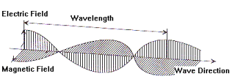
where
h is Planck’s constant (6.626 x 10⁻³⁴ Js).
Electromagnetic energy with a large wavelength and short frequency (for example,
microwaves) consists of low energy photons, and visa-versa. The electromagnetic
spectrum is divided for convenience into order of increasing frequency and
consequently decreasing wavelength. The energy level of the photons the
frequency and wavelength of the wave all interact to determine the wavelength
dependent interactions with materials at the Earths’ surface, and hence the
information content of the data.
|
Figure 3. 2 shows the wavelength regions that are used to remotely sense soil properties. They include both physical and chemical properties that have either a direct or indirect effect on the amount of EM radiation reflected from an object (Clark & Roush, 1984). Photons arriving at the materials surface are reflected from the materials external and internal surfaces reflected or absorbed by the material (Figure 3. 3). Reflection and scattering vary with the geometric properties of the surface. Absorption is the retention of radiant energy by a
substance caused by the transformation of radiant energy into heat
(shorter to longer wavelength). |
Figure
3. 2.
A division of the electromagnetic spectrum into regions, showing their
frequency in Hertz and potential for proximal (and remote) sensing of
various soil properties, including potassium (K), soil colour (SC), soil
organic matter, clay content including iron (CC), soil nitrogen (SN),
cation exchange capacity (CEC), soil water (SW), and soil
structure – soil strength measurements (SS). (Adapted from
Viscarro-Rossel & McBratney 1998.) |

It is described in Beers’ Law by the absorptivity el.
Absorption features are the result of physico-chemical phenomena occurring
at a molecular level including intermolecular vibrations and electronic
transitions within atoms.
Electronic processes
require high-energy photons and occur in
the UV, VIS and NIR wavelengths. Electromagnetic energy is either emitted or
absorbed when an atom or molecule changes from one energy state to another.
Absorption of photons of a specific wavelength causes a change from one energy
state to a higher one. Emission occurs as a result of a change in energy state
from a higher to a lower one. When a photon is absorbed it is usually not
emitted at the same wavelength. There are three ways in which electrons can be
moved from one energy level to another, the most important are charge transfer
absorptions.
|
Figure
3. 3.
Possible interactions of electromagnetic energy with a
material. |
Charge transfer absorptions, and inter-element transitions, result in
absorption when a photon causes an electron to move between ions or
between ions and ligands. Transfers are possible between ions having
different valence states (i.e. Fe2+, Fe3+). Small
shifts in absorption band positions can occur due to the substitution of
other elements, such as aluminium for iron in hematite. Charge transfer
absorptions are important in discriminating between soils. Fe-O charge
transfers are particularly notable in the blue and ultraviolet wavelengths
(<0.6mm). The change of slope of reflectance spectra in
this region is normally considered to reflect differences in organic
matter and iron content. Crystal field effects
cause weak absorption features in
minerals. Transition elements (Ni, Cr, Co, Fe, etc.), Fe being dominant in
soils, have unfilled electron shells. The d orbitals of individual
isolated ions of each of these transition metals have identical energies,
but when the atom is located in a crystal field the energy levels split.
That is, the energy levels of the d orbitals vary. Electrons can then
be shifted from one energy level to another by absorption of a photon
having energy matching the energy difference between the
levels. |
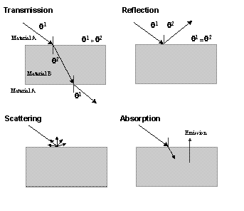
The
valence of the atom, its co-ordination number and the symmetry of the site it
occupies within the crystal define the energy levels. The crystal field varies
with crystal structure from mineral to mineral, the same ion producing different
absorptions. Crystal field effects are weak in comparison to charge transfer
absorptions.
Conduction bands occur when electrons may reside in two energy levels, the ‘valence’ band, a lower energy region where electrons are attached to individual atoms and a higher energy ‘conduction’ band. Electrons occupying the conduction band may flow freely through the mineral lattice. The difference between the two energy levels is the ‘band gap’. The band gap is only of significance for dielectric materials such as sulphur, where it causes the distinct yellow colour.
Occurring in wavelengths typically greater than 1mm (low energy), vibrational processes involve atomic resonance, harmonic motion and bending. The bonds in a molecule or crystal lattice can be considered to be like springs with attached weights. With an input of energy at the correct wavelength the whole system can vibrate, bend and stretch. The frequency of the vibration depends on the strength of the bonds and the masses of the elements in the molecule or crystal lattice.
Texture differences cause major changes to the shape of reflectance spectra for two reasons, a) the properties of the solids having characteristic particle sizes (clays/sands), such as transmissivity and absorption and b) the strong relationship between texture and soil composition. In theory, the reflectance of a granular solid should increase across all wavelengths, as the particle size decreases (Clark and Roush, 1984). Larger grains have longer internal path lengths over which photons may be absorbed. Smaller grains have a much larger surface area to volume ratio so there are many more possibilities for surface reflections and multiple scattering. The optical path of the photons is that of a random walk. A bright material, having low absorption and high transmittance and typically large grains (i.e. sand), will allow photons to continue their random walk. At each encounter with a grain a small percentage will be absorbed. So, weaker absorption features will be better expressed (Palacio-Orueta et al. 1998). Soils with a sandy texture tend to have smaller amounts of organic matter, iron oxides and clay minerals, which are dark, strongly absorbing opaque materials. Small amounts of these materials and a high overall reflectance combine to cause their absorption features to be better defined in sandy soils than in clay soils which have larger contents (Soares Galvao et el. 1996).
Organic matter in soils consists of unaltered or partially
altered biomass (plant residues and micro-organisms) and humus. It is therefore
a mixture of many different compounds and biomolecules. A unique
characterisation of their spectral properties is not possible. In general,
organic matter reduces reflectance across the whole 400 to 2500 nm region
(Hoffer & Johannsen, 1969) and causes a reduction in the slope and a concave
or linear shape to the spectrum within the 500 nm-800 nm region (Latz
et al. 1984). It dominates the soil spectrum when in excess of 2% of the total
soil mass, masking the absorption features of the soil minerals, reducing the
resolution of the absorption bands (Soares-Galvao et al. 1997). However, with
the appropriate analysis absorption features caused by specific carboxylic and
amide groups present in the organic matter fraction can be identified (Janil
& Skejmstad, 1995a b).
Clay minerals cause a minor
absorption band at 2.2-2.3mm
that is often diagnostic for soils (Stoner & Baumgardner, 1981). Absorption
features between 2.1 and 2.2mm
often relate to a combination of –OH stretching and Al-O-H bending modes, which
are characteristic of dioctahedral clays (i.e. kaolinite). The metal bending
mode at 2.3mm
may reflect the presence of Mg-O-H bonds, typical of trioctahedral clay
minerals, for example smectite (Pieters et al, 1993).
Iron
in soils decreases reflectance across the whole spectrum, but at wavelengths
beyond the visible region the reduction in intensity is more acute (Stoner &
Baumgardner 1980). Absorption features short of 1000 nm are due to iron
oxide phases. At 950 nm ‑ 1000 nm ferrous iron presence is
indicated by a subtle and broad absorption feature, while in the region of
650 nm, ferric iron causes a steep fall off (concavity) from the red to the
blue wavelength (Soares Galvao et al. 1997).
Water
causes strong absorption bands at 1.4mm and 1.9mm (most sensitive), with weaker bands at 0.97mm, 1.2mm and 1.77mm. They are the result of overtones and combinations of the
three fundamental vibrational frequencies of the H2O molecule. In
soils where the water is in an unordered state the bands at 1.4mm and 1.9mm are often broad. Soils typically exhibit distinct
absorption bands at 1.4mm, 1.9mm and 2.2mm due to the presence of –OH bonds, either in the soil
mineral (at 1.4mm and 2.2mm) or in the water molecule itself (at 1.9mm). Hydroxyl stretches occur at 1.4mm. Combinations of –OH stretches and an H-O-H bend occur at
1.9mm. Therefore, a mineral with a 1.9mm absorption band contains water (halloysite, for example),
whilst a mineral with absorption band at 1.4mm but no 1.9mm band has only a small amount of water, yet a large amount
of –OH, for example kaolinite (Clark & Roush, 1984).
The
shape of a soil spectral curve in the visible range does not change shape as a
function of wetting. The ratio of the wet soil reflectance to the dry soil
reflectance remains constant. Increased water content decreases the reflectance
of soil samples, because drier soils have a greater number of air filled pores
that increase the amount of backscattering radiation (Viscarro Rossel &
McBratney, 1998).
Colour, the perception of EM
energy
Historically observations of soil
colour were the only way to measure the EM reflectance properties of soils.
Colour describes the human perception of light energy coming from an object, by
the retina. The retina is composed of three types of cone cells that act as
photoreceptors. For this reason three attributes are necessary and sufficient to
describe a colour; Hue, lightness and saturation. Each cone cell is sensitive to
light of different wavelength regions (Figure
3. 4) between wavelengths 380 nm and 770 nm (Wyszecki
& Stiles, 1982). Three factors interact to determine the colour observed:
(i) The spectral power distribution
of the light source, i.e. the illumination conditions.
(ii) The spectral reflectance
characteristics of the object (as measured by a
spectrometer).
(iii) The sensitivity of the eye
(or other measuring device).
The colour sensation perceived by
the eye - brain combination is specific to each individual and circumstance.
Each light source, for example the sun or a lamp, has a characteristic relative
power at each wavelength within the visible spectrum. When field sampling
daylight conditions change throughout the day and as a result an objects
reflectance and the perceived colour vary throughout the
day.
|
It is recommended that
observations of colour be made under standard illumination conditions, for
example Source C, an approximation to daylight quality (Melville &
Atkinson, 1985). While Kelly & Judd (1976) suggest that an experienced
observer can identify the subtlest of colour variations and match them to
the correct chip when in a viewing booth, each observer is unique and the
process of human vision complex and poorly
understood. For these reasons spectral
reflectance measurements made under standard laboratory conditions, on
prepared samples, by a spectrometer offer a clear advantage over
measurements made by observation (Fernandez & Schulze 1987, Post
1993). Colour is a sensation and therefore the language used to describe
colours is also highly specific to the individual and can therefore be
hard for others to interpret |
Figure
3. 4.
A possible reflectance spectra for the visible part of the electromagnetic
spectrum. |

To facilitate the transfer of
colour data and information between individuals and appliances, formalised
colour order systems have been developed. A colour order system describes an
orderly three-dimensional arrangement of colours. There are three bases used to
order colours: 1) an appearance basis, such as the Munsell system of Hue
(dominant wavelength), Value (lightness) and Chroma (saturation); 2) an additive
colour basis (such as the CIE and RGB systems), and 3) a subtractive
basis (cyan, magenta and yellow system). An optimal colour system is one that
describes a uniform physical and perceptual colour space and is described by
linearly scaled equi-dimensional variables (MacAdam, 1981) that facilitates the
identification, numerical representation and interpretation of colour
differences.
An
appearance basis: the Munsell colour notations
The Munsell System of Colour
Notation is a colour order system invented by an artist Albert H. Munsell in
1905, prior to the development of a quantitative means of measuring colour. It
specifies a limited number of 'standard' colours, within a 'cylindrical' colour
space. Three attributes, Hue (H), Value (V) and Chroma (C) describe the
similarity to a dominant colour (red, yellow, blue) or a combination of any two,
the colour intensity (lightness or Chromaticity) and the relative purity of the
dominant wavelength or perceptual difference from a neutral grey (saturation)
respectively.
|
(a) (c) Figure
3. 5.
(a) Munsell Hue (b) Munsell Value,(c) Munsell Chroma (colour wheel) and
(d) the complete Munsell colour system, showing the non-uniformity of the
Chroma axis. |
In the Munsell soil colour
charts, Hue takes eight categorical values: red (10R), red- yellow (2.5YR,
5YR, 7.5YR, 10YR), yellow (2.5Y, 5Y). For visualisation purposes they are
arranged in a circle or cylinder (Figure
3. 5a + d) following the natural order of Hues.
Black, white and the intermediate greys have no Hue. They are achromatic
(R=G=B), and with a separate code.
=The Munsell attribute Value (V) varies in value between 0 and 28
(only 0-8 are used in soil chart). Value represents changes from black to
white (Figure
3. 5b) and variations can be visualised as shifts
along the vertical axis of the Munsell cylinder. Chroma varies between 0
and 9. Changes in Chroma can be thought of as being the result of the
addition or subtraction of a neutral grey (Figure
3. 5c), and variations represented visually as
changes in the distance from the central axis of the cylinder (Figure
3. 5d). The scales of Value and
Chroma were intended to be graded such that each step was perceptually
equal, but not such that the scales of the two variables vary
equi-dimensionally, i.e. 1:1. Melville & Atkinson (1985) show that
while these two variables are independent, therefore error in assigning
one does not affect the other, that in reality there is a 2.5 : 1 linear
ratio between the scales of the two
variables. |
 (b)
(b)


A psychophysical basis of additive
primaries: the CIE and RGB colour
systems
Human colour vision obeys the
principle of superposition. Psychophysical additive colour systems are based on
the same principal; the values of the variables describing the colour are
proportional to the light intensity. When the three variables describing the
colour sum to 100 % intensity, white light is produced. Combinations of the
three variables in varying intensity produce a range of colours or gamut (Figure
3. 6). The variables are linearly independent therefore
the colour produced by any additive mixture of three spectra of primary colours
(for example red, green and blue primaries) can also be represented and
predicted by adding fractions of corresponding components of the primary
spectra. This means, a colour that can be mixed from a combination of pure
primaries, can be generated by combining other colours, the combination of which
represents an equivalent combination of the pure
primaries.
|
In 1931 the CIE or Commission
Internationale de l'Eclairage standardised the description of colour by
specifying the light source, the observer and the methodology used to
derive the colour space coordinates (CIE, 1936). In the CIE system the
dominant Hue is a function of the relative intensity of the reflectance of
the object at each wavelength and the wavelength dependent sensitivity of
the eye to light energy, which is most acute at 550 nm (Wyszecki &
Stiles, 1982). |
(a)
Figure
3. 6.
Additive colour combinations within the RGB colour space. Illustrates how
different real RGB primaries generate different colours when combined in
the same proportions. |

The Luminance of the object is a
function of the total intensity of the light energy. The perceptual response to
Luminance is defined as lightness. The third attribute, the saturation, is the
colourfulness of an area judged in proportion to its Luminance. So while the
phsycophysical colour order systems are represented by continuous variables that
have numerical properties favourable for multivariate statistical analysis, such
as independence and uniformity of scale, they can also be used to provide a
description of colour in perceptual terms analogous to those provided by the
Munsell code, namely Hue, Value (lightness) and Chroma
(saturation).
|
(a) (b) Figure
3. 7.
(a) CIE colour matching functions and (b) spectral power distribution for
the Standard Illuminant C. Required for transformation of reflectance
curves into colour coordinates |
CIE
tristimulus coordinates.
The CIE system defines how to
map a spectral power distribution R (l) to a set of tristimulus
coordinates that describe this colour space; a Luminance component Y,
described above and two other 'imaginary' primary spectra X and Z. The
term imaginary refers to the fact that neither corresponds to a defined
colour, for example red, green or blue. The sensitivity of the human eye
to variations in X and Z has been measured to provide colour matching
curves (Figure
3. 7a, CIE, 1931) which relate the magnitudes of
X, Y and Z to the physical energy emitted at a given wavelength in the
visible portion of the spectrum. Spectra
R (l), collected in the laboratory
can be transformed to the CIE coordinates by Integration with colour
matching functions ( Equation 3. 3
The Y attribute is
conceptually similar to Munsell Value, but X and Z do not have any
physical meaning. The magnitudes of the XYZ components are linearly
proportional to physical light energy, but the spectral composition that
they represent depends on the colour matching characteristics of human
vision, thus the values of XYZ are difficult to
interpret. CIE trichromacity
coordinates
The tristimulus values can be
transformed into chromaticity coordinates to provide a graphical
representation of the colour space that is easier to conceptualise and
interpret. The chromaticity triangle is a projection of the chromaticity
coordinates into the red-green plane (Figure
3. 8a). |
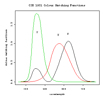
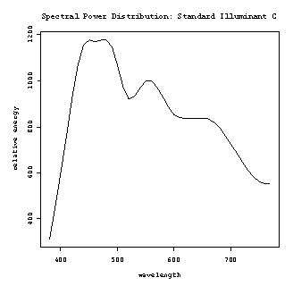
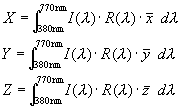
Equation 3. 4
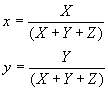
Because x + y + z, sum to 1
only two of the variables are necessary to describe the colour differences under
standard illumination conditions. Each variable is non-negative and must lie
within the bounds [0,1]. Given the Luminance Y and the Chromaticity coordinates
x y, the XYZ tristimulus values can be recovered (Escafadel,
1993):
|
A chromaticity diagram is
invaluable for the interpretation of colour differences and for relating
the colour systems one to another (Figure
3. 8b). The chromaticity diagram shows a rounded
cone bounded by the saturated 'pure' colours (Mattikalli, 1997). The
boundary of the cone is called the locus spectra.
|
(a) Figure
3. 8.
(a) Mapping of XYZ tristimulus values to (b) an x y Chromaticity
Diagram. |
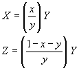
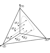
Within this space each point
designates a unique colour with reference to the illumination and viewing
conditions. The achromatic point corresponds to the reference illumination
colour (Mathieu et al 1998). The third coordinate Luminance can be imagined as a
pyramid-like volume. At the apex, 0 % Luminance represents black, while the
base, 100 % Luminance corresponds to pure white. The values of x and
y cannot be related directly to the Hue and Chroma of the Munsell system.
The x value represents variation from blue to red and that of y,
blue to green. Coordinate interpretation and therefore colour visualisation are
provided by reference to the chromaticity diagram, although, even with
experience, the imaginary basis of the system means that it is difficult to
visualise a colour from a knowledge of the trichromaticity coordinates xy
alone.
CIE
L* a b system
The CIE
XYZ system has drawbacks. It is difficult to represent the Luminance
graphically, but more importantly there is a discrepancy between perceived
colour differences and the actual spacing of the perceived colour in the
system.
|
(a) Figure
3. 9.
The CIE xy Chromaticity diagram (a) and the CIELUV Chromaticity diagram
(b). Each line represents a colour difference of equal
proportion. |
The values of the coordinates
are uniformly proportional to the light energy, but are non-uniform in
perceptual colour space. This is illustrated by Figure
3. 9a where the bars represent a colour difference
of equal perceptual magnitude. More recent attempts by the CIE to improve
the perceptual representation of a continuous metric colour space, have
resulted in the CIE L* a b and CIE L*u v colour spaces
(MacAdam, 1985). The CIE L*u v system
was first used in soil science by McBratney & Webster (1981) and
Burrough (1983), however Melville & Atkinson (1985) remark that
despite what are only small differences between the two systems that the
CIE L* a b coordinates are more uniformly related to the Munsell
coordinates. Therefore we focus on this system and do not present any
details of the CIE L*u v space. |
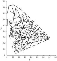
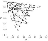
The CIE L* a b system is described by the Luminance coordinate L*, and two Chromaticity co-ordinates a and b. Together they describe the differences of the three elementary colour pairs: red-green represented by changes in the value of a, yellow-blue by b (Figure 3. 10) and black-white, by L.
|
The L*a*b* values are
calculated by a non-linear transform of XYZ (Equation 4) with reference to
the XYZ values of the aChromatic colour, C. Using standardised XYZ values
(xyz) the CIE L* a b coordinates are given by, |
(a)
Figure
3. 10.
(a) A simple 3-D representation of the CIELAB system and (b) a 2-D
representation of a CIELAB colour plane of equal
Luminance. |
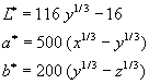
The CIE L* a b coordinates describe
a colour space wherein perceived colour changes are almost linearly related to
the magnitude of changes of light intensity (Figure
3. 10b), meaning that perceived colour differences can be
related more easily to changes in the values of the Chromaticity coordinates.
Nevertheless, the basis of the CIE L* a b system is unfamiliar to soil
scientists and unlikely ever to be used during qualitative
surveying.
The RGB system
The
RGB system is based on the same concept of additive primaries on which
the C.I.E. XYZ system is formulated, however the use of real primary spectra
such as those of red, green and blue primaries, instead of the imaginary XYZ is
generally considered to provide a more physically interpretable colour space
(Escafadel 1993, Mattikalli 1997). Combinations of the primaries are easier to
imagine, therefore the individual values themselves are potentially easier to
interpret (Figure
3. 11a+b). The colour space is constructed in the same way
as the CIE system, by integration of primary spectra with the measured
reflectance R (l) and the wavelength dependent power
of the illuminant I (l),
Equation 3. 7
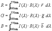
It is also possible to standardise
the variables using Equation 3. 5. The rgb trichromaticity coordinates can be
plotted in a colour triangle of equal Luminance and analogies drawn between the
RGB, CIE Y xy and Munsell colour spaces (see next section). The range of
colours that can be produced by combining primaries depends upon the Chroma of
the RGB primary spectra used.
|
An example is shown in the
xy chromaticity diagram by the triangle whose vertices are the
chromaticities of the r g b primaries (Figure
3. 11a). While the range of possible colours is
less than that described using the XYZ primaries, combinations of red,
green and blue spectra can produce the largest range of colours of the
real primaries (Wyszecki & Stiles, 1982). Unfortunately, equal variations of the each of the RGB values do not represent an equivalent change in the perceived colour towards one of the primaries, because the eye is more sensitive to variations in the intensity of the green primary component than the red or blue. The RGB colour space is therefore numerically uniform but perceptually non-uniform. |
(a) Figure
3. 11.
(a) the RGB gamut in 3-D and (b) a 2 dimensional RGB gamut showing that
linear combinations of the primaries produces the range of possible
colours. |
 (b)
(b)
Psychophysical colour spaces: Hue,
saturation, lightness
While each of the modern colour
spaces offers certain numerical advantages over the Munsell code, none provides
the interpretability of the Munsell colour attributes. To provide attributes
with similar meaning the coordinates of each of the quantitative colour spaces
can be further transformed to provide a perceptual description of colour in
terms of Hue, Saturation (Chroma) and Lightness (Value), that are analogous to
the Munsell colour space. For example, the edges of the RGB triangle
represent the pure colours. The achromatic vector (illuminant white) is equal to
the line R = G = B. The RGB Chroma is represented by the relative length
of the vector from the achromatic centre to the point representing the colour,
while the Hue is described by convention as the angle formed by this vector and
the axis running from the blue vertex to the yellow midpoint (Escafadel 1993).
Similarly, the CIE L* a b coordinates can be transformed to CIE Hue and Chroma
values,
Equation 3. 8
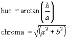 .
.
They facilitate visualisation of
the colour within the CIE L* a b spherical colour space (figure 7b) and describe
the same perceptual changes as the Hue and Chroma attributes of the Munsell
system. They provide an important advantage over both the Munsell and rgb
representations because the CIE L* a b colour space is described by linear
independent variables that are both numerically and perceptually
uniform.
Starting from a C.I.E chromatic
representation of colour, Mathieu et al (1998) transformed the trichromaticity
coordinates xy into the Helmholtz coordinates; the dominant wavelength
ld, and purity of excitation Pe %,
which are analogous to the Munsell and CIE L*a b Hue and Chroma
respectively. The dominant wavelength (Hue) is the value of the locus spectra at
the point described by the line which passes from the achromatic point C through
the point defined by the chromaticity coordinates, M(x,y). The purity of
excitation (Chroma) represents the proximity of M(x,y) to ld and is calculated as the ratio of
the distance CM / Cld.
Methods and analysis
Spectral reflectance measurements
The spectral reflectance properties of 110 soil samples were measured in the laboratory using a Varian Cary 5e UV/VIS-NIR spectrometer (limiting resolution005nm). Each sample was dried, crushed and sieved (<2mm). To remove any unwanted effects of aggregation on reflectance. The spectrometer was fitted with an external sample holder from which all ambient light was excluded.
|
A specially designed sample
holder was made that permitted the soil to be poured in so that the soil
lay flat against the glass surface through which the spectrometer
measures. A lid was then slid over the sample and the holder turned over
to face glass side up. This reduced irregular surface roughness that would
introduce unwanted variability to the measurement process. The capability
of a spectrometer can be described by several sensor specific parameters,
for example the resolution and signal to noise ratio (see Box 3), which
combine to determine its ability to identify a given material or resolve a
specific problem. Each spectral curve consisted of 1065
measurements between 250 nm and 2500 nm with a resolution of
0.01 mm,
(~3 nm FWHM). |
Figure 3. 12. Schematic diagram of a double beam
spectrometer |
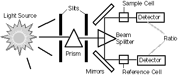
|
|
With 1065 contiguous individual wavelength measurements it is highly probable that much information is repeated and that many of the individual bands contain data that is redundant. It is common practice to reduce the number of bands to a number sufficient for the specific objectives of the analysis. Hyperspectral imaging sensors such as AVIRIS or HYMAP collect approximately 220 to 250 individual wavelength measurements with a resolution (FWHM) of 10nm. This is largely sufficient for soil studies. Palacios-Orueta & Ustin (1996) convolved laboratory spectral reflectance measurements to the AVIRIS data format and compared the information content of the two datasets. They then used principal components analysis to further reduce the number of explanatory information containing variables before using these to predict the properties of the soil. Principal components transforms a set of correlated quantities into uncorrelated factors under the constraint that factors successively represent a maximal amount of the variance. The factors are called principal components (PCs). Each principal component is calculated as a linear combination of an eigenvector with a standardised variable (Wackernagel, 1997). The eigenvectors or loadings represent the amount of variance each variable explains along the axis represented by the PC in the transformed space. The component scores give the location of each sample in transformed space. The amount of variation expressed by each axis, the eigenvalues, can be expressed as a percentage of the total variance of the data. There are as many underlying factors as there are variates in the data. Usually only the first few that account for the majority of the variance (~90-95 %) are kept. The others are discarded, and as a result the data dimensionality has been reduced. |
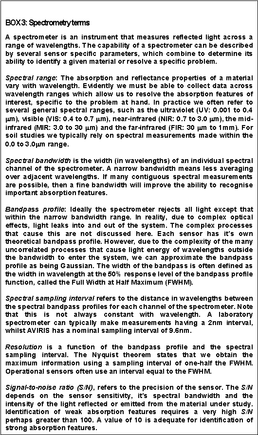
Colour transformations are an alternative means of reducing the amount of data that are explored here. The analyses of the spectral reflectance data consisted of 3 stages:
1. Initial reduction of data by convolution to degraded format
· The 1065 (3nm FWHM) measurements collected on 110 samples of the 0-10cm soil layer convolved to 252 (10nm FWHM) using a triangular bamndpass (code in appendix).
· The information content of these two datasets was compared by transforming to principal components and comparing their factor loadings.
2.
Transformation of the spectral reflectance data to colour representations.
Transformation of observed colour in the field, represented in Munsell
coordinates to other colour spaces.
- Munsell values provided by colour matching in the field and spectral reflectance curves collected in the laboratory were both transformed into CIE XYZ and RGB tristimulus coordinates (Munsell Conversion Software V 4.01), then standardised to provide the compositional CIE xyz and rgb trichro aticity variables.
- The CIE XYZ values were also used to calculate the CIE L* a b, Hue and Chroma coordinates (Equation 3. 6) to provide a perceptual representation of the quantitative colour spaces that could be related to the Munsell attributes.
3. Multiple linear regression (MLR)
models were used to evaluate the potential for the use of spectrally derived
colour to predict soil properties.
·
Spectrally derived colour
coordinates replaced the observed values of colour in the fuzzy classification
presented in the chapter 1. The results of the two classifications were compared
to see whether they summarise similar soil information.
· Spectrally derived colour in each format was regressed against soil properties, to i) identify the optimal colour space representation and ii) to indicate the improvement in prediction quality that is attainable if visual observations were replaced by quantitative measurements of colour.
Results
The spectral reflectance curves showed many of the characteristics typical for soil. Absorption features are deeper and better defined for those soils with a larger sand content. Figure 3. 13 shows two spectral reflectance curves, characteristic of (a) the Red and (b) the Cotton soil. The major differences occur at wavelengths < 600 nm and at 900 nm. The Cotton soil curve is convex across this region. The Red soil curve is concave as iron coating the surfaces of the sand grains causes absorption. The effect of a higher sand content is also evident from the slightly deeper absorption band at 1400nm and 1900 nm most likely the result of water ( ‑ OH).
|
(a)
(b) Figure
3. 13.
Examples of spectra with median loading on factors 1, typical of a Red
soil (a) and factor 2 , typical of a Cotton soil (b) [solid black line],
with interquartile range [dashed line]. |
The principal components of each dataset containing 1065 and 252 individual measurements were the almost identical (Figure 3. 14 and Figure 3. 16). Reducing the number of variables from 1065 to 252 by convolution to the AVIRIS spectral resolution did not reduce the information content of the data, illustrating that there is much data redundancy in the complete laboratory spectra dataset. Further analyses could be speeded up and simplified somewhat by using the smaller dataset. |
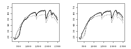
|
The principal component loadings for both data sets revealed the same features. Principal component 1 (Figure 3. 16a and e) loaded positively for concavity of the spectra in the 250-400 nm region and negatively for longer wavelengths. The second principal component weighed (Figure 3. 16b and f) positively at 1900 nm and again near 2200 nm, absorption bands for Al‑OH and –OH bound between clay lamellae. Both of the first two principal components loadings showed a peak or trough near 950 nm, an absorption band for ferrous iron. |
(a)
(b) Figure
3. 14.
Screeplots (a) number of wavelengths = 1065, (b) number of
wavelengths = 252 equivalent to AVIRIS sampling interval and
FWHM. |
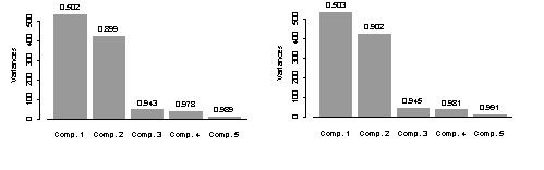
|
Figure
3. 15.
Samples plotted in the space of component scores (a) components 1 and 2,
(b) components 2 and 3, both show a partition of according to soil type
(as indicated by letters: C = cotton soil, R = red,
T = transition and A = levee), and (c) components 3
and 4, that does not. |
The third principal component (Figure 3. 16c and g) had positive loadings at 1400 nm and 1900 nm. Both absorption bands correspond to the presence of –OH bonds, either in the soil mineral or in the water molecule itself. Principal component four had low information content, with all loading values nearly zero. Plots of the component scores
the orientation of the samples relative to the transformed axes (Figure
3. 15a), show that the first two principal
components group the soils according to whether they are of Red or Cotton
type. Lower order PCs 3 and 4 do not distinguish between the soil
types. |

Comparing colour space
representations and the effects of measurement
quality
The
Munsell values provided by colour matching auger samples while surveying
(0-10cm, 30-40cm, 70-80cm and 90-100cm) and spectral reflectance curves
measured on the 110 samples in the laboratory (0-10cm layer only) were
both transformed into CIE XYZ and RGB tristimulus coordinates. The
Munsell values were converted using the Munsell Conversion Software V 4.01
freely available from the internet. The
spectral curves were transformed using code provided in the appendix. The
CIE XYZ and RGB tristimulus coordinates were then standardised
(Equation 3. 2) to provide the compositional CIE xyz
and rgb trichromaticity variables. The
CIE XYZ values were then used to calculate the CIE L* a b, Hue
and Chroma coordinates (Equation 3. 6) to provide a perceptual representation of
the quantitative colour space coordinates that could be related more
easily to the Munsell attributes. The results of the analyses of the
observed colour data are presented first. The spectrally derived colour
data is then considered. Observed colour: coordinate
representations
It is possible to analytically transform from Munsell coordinates to any other colour space (Mattikalli, 1997). However, the coordinate values of the CIE XYZ and RGB colour spaces are not designed to relate to one another meaningfully. |
Figure
3. 16.
Eigenvectors of the first four principal components of the reflectance
curves (a-d) number
of wavelengths = 1065, (e-f) number of
wavelengths = 252 equivalent to AVIRIS sampling interval and
FWHM. |

The
relations between the Munsell and CIE Yxy colour space are non-linear.
Scatter-plots of corresponding colour space coordinates were not informative
(Figure A4 2), because the physically interpretable variation represented by a
single 'perceptual' (or psychophysical) Munsell coordinate was factorised
between the imaginary primary components, XYZ.
|
Figure
3. 17.
Scatterplots of Munsell Hue, Value and
Chroma and CIE L* a b
Hue, Luminance and Chroma analogs, showing the 1:1 relation between the
colour space representations. |
As a
result, there was no clear grouping of points in the plots according to
soil type. Only the CIE Y and Munsell Value coordinates were linearly
related to one another, because they have similar physical meaning, both
representing changes in luminance (the intensity of the lighting
source). There was an almost 1:1
correlation between the Munsell Hue, Value and Chroma coordinates and the
equivalent CIE L* a b psychophysical coordinates (Figure
3. 17). Therefore, it was possible to relate one to
the other numerically and perceptually and thereby benefit from the
advantageous properties of the latter during statistical analysis, whilst
retaining the same perceptual framework of Hue, Value (Luminance) and
Chroma with which soil experts are familiar. The
relations between Munsell Chroma and the red and blue coordinates, and
Munsell Value with green were also readily interpreted (Figure A4 3). They
suggested that variation along the red - blue axis caused changes in the
saturation or relative purity of the dominant soil colour, while the
lightness of the soil colour was strongly linked to the intensity of the
green primary, to which the eye is most
sensitive. |

Observed colour: changes with
depth
Figure
3. 18 and Figure
3. 19 show the distribution of colour coordinates for each
soil type with depth, for the Munsell and rgb systems. Meaningful
information can be derived from each colour space representation by interpreting
first the coordinate space with which we are most familiar (Munsell), then by
interpreting observed trends with depth for the other colour spaces in light of
these findings and with reference to our conceptual understanding of how soil
properties affect the observed colour, for the soils of the
region.
|
Levée and Cotton soils have
identical Hue (10 YR) throughout the soil profile (Figure
3. 18). The Red soil is a mix of 2 YR and 5 YR. The
full range of Hues is expressed by the Transition soil because as its name
implies this class is spatially located along the boundaries of Red and
Cotton soils and represents a gradation from one to the
other. The distribution of Chroma
divides the pedon classes into two groups; Red and Transitional, Cotton
and Levée. The former have a positively skewed distribution (mode = 2),
the latter negatively skewed (mode = 6). The distributions of Munsell
Value divide the classes similarly. Variability of Munsell Value within
the Levée class is probably caused by the heterogeneity of the dominant
grain size of materials deposited close to the rivers edge, and from which
these soils are formed. Soil texture plays an
important role in determining the total amount of light energy
backscattered by a soil (Viscaro-Rossel & McBratney, 1998) and
therefore can affect considerably the perceived lightness of the
soil. The Red/Transitional and the
Cotton/Levée soil grouping are clearly illustrated in Figure A4 6, which
shows the CIE Yxy distributions with depth. Chromaticity values
(xy) are largest for both the Red and Transition soils at all
depths. However, the difference between the average values of each class
decreases with depth.. |
Figure
3. 18.
Box and whisker plots showing the changes in observed Munsell Hue, Value
and Chroma with depth for 4 soil layers (0-20 cm,.30-40 cm,
70-80 cm and 90-100 cm). The width of the boxes is proportional
to the number of observations in each soil type (A = Levée, C =
Cotton, R = Red and T = Transition
soil types) |
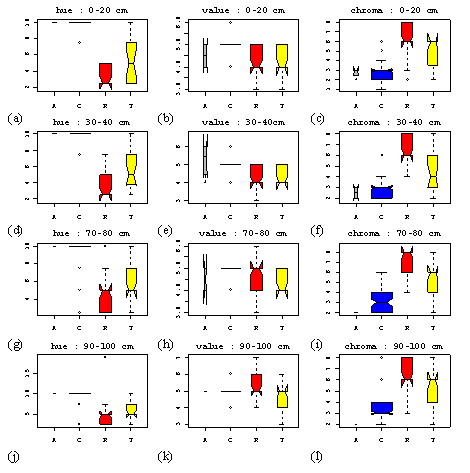
|
Figure
3. 19.
Box and whisker plots showing the changes in observed red, green and blue
coordinates with depth for 4 soil layers (0-20 cm,.30-40 cm,
70-80 cm and 90-100 cm). The width of the boxes is proportional
to the number of observations in each soil type (A = Levée, C =
Cotton, R = Red and T = Transition
soil types). |
Other variations with depth
include a shift from high to lower values of Luminance for Cotton and
Levée soils, while the change is in the other direction for the Red and
Transition soils. This could be interpreted as reflecting the vertical
distribution of salts in the profile. Carbonate and gypsum accumulations
were common at depth (between 60 cm and 80 cm) in Red and Transition soils
and uncommon in Cotton and Levée soils. While observable salt
concretions were less common for the latter, these soils are prone to
salinity-sodicity. The accumulation of such white coloured soluble salts
in the surface layers of the profile may have increased the perceived
lightness, while not being directly observable as
concretions. The
rgb colour space distributions were consistent with these
observations (Figure
3. 19). Red and Transitional soils have
significantly larger values of the red primary at all depths, while Cotton
and Levée soil have larger values of the blue and green primaries. The Red
soils are indeed redder and the Cotton soils bluer; the result of
differences in texture and soil water regime. The range of rgb
values of the 30-40 cm layer is small, in stark contrast to those at all
other depths. This feature is common to all classes and tristimulus
values, but is most marked for the green coordinate and in general for the
Cotton soil. This soil was invariably under cultivation and suffered from
compaction and anaerobic conditions, that gave rise to a hard, grey
soil. |
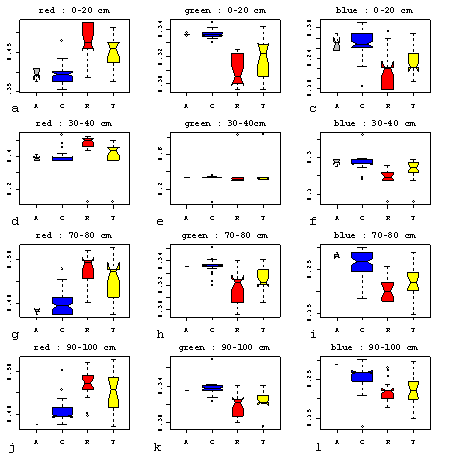
Spectrally derived colour:
Transformations
The
divisions of the Munsell code mean that the transformation of a coordinate
from this space to a continuous counterpart is many-to-one. Not
surprisingly, the continuous representations derived from the colour
matched Munsell values and presented in the previous section are unclear
and difficult to interpret. Plots of the observation (colour matching)
derived colour coordinates against those derived from the measurements of
diffuse spectral reflectance (0-10cm soil layer, Figure
3. 20) illustrate the effects of the method of
measurement on the relationships between the two. Coordinates that describe the
Luminance (Value for Munsell, Luminance for CIE L* a b, y
for CIE xyz and g for the rgb colour space) are
understandably most affected by varying illumination conditions (Figure
3. 20). The dispersion of the values of each of the
coordinates describing luminance obtained by colour matching, far exceed
the range of the spectrally derived colour coordinate
values. |
Figure
3. 20.
A comparison of colour coordinates derived from observations made in the
field and those calculated from spectral reflectance measured under
laboratory conditions. |
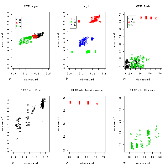
The reason for this observation is
clear: the illumination conditions and sample preparation varied more when
colour matching in the field, than when measuring reflectance under standard
illumination conditions and with uniform sample preparation in the laboratory.
With the exception of the CIE L* a b Hue and Chroma coordinates the
relationships between colour matched and spectrally derived coordinates, while
coherent, are weak.
Spectrally derived colour:
Chromatic representations
The chromaticity derived from the
spectral reflectance measurements (Figure
4. 1), provided a clear graphical repartition of
samples according to soil type, testament to the importance of soil colour when
allocating samples to a soil type and the validity of colour matching to
correctly distinguish between soils when in the field.
|
Figure
4. 1.
Plot of the spectrally derived xy colour coordinates, showing the soil
type allocation. |
The
origin of the chromaticity diagram (a) corresponds to the chromatic point
of the standard Illuminant C. The arrows indicate the dominant wavelength
of selected samples, and the horizontal and vertical lines possible
cut-offs for a rapid colour based classification of the samples into the
two modal soil types. Red and Transition soils are
grouped close to the achromatic point along a vector corresponding to a
dominant wavelength of 580 nm (towards the Red primary). In contrast the
slope of the vector along which the Cotton soil samples lie, indicate a
dominant wavelength of 560 nm (towards the Blue primary). These plots show
how soil colour varies continuously. At the simplest level of
prediction, these values could be used to allocate additional samples from
the region to either of the modal soil types (Cotton or Red), by applying
a cut-off to the either xyz or rgb values. If a spectrometer is not
available the colour measurements could be made by cheaper means, such as
a portable colorimeter. |
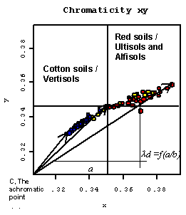
Correlations between colour space
variables and soil physical and chemical properties
The spectrally derived colour
measurements were used to predict other soil properties, and to evaluate the
potential improvement in prediction quality permitted by replacing qualitative
observed colour data with quantitative measurements of colour. It was necessary
to define which colour space coordinates correlated best with selected soil
properties, given the lack of consensus amongst soil experts as to which offers
the greatest advantages.
|
Table
3. 1.
Correlations between colour coordinates, from in-situ colour matches and
spectral reflectance measurements and selected soil properties, for which
a reasonable correlation was observed. *Indicates significant correlation
(0.05 level). n/a refers to correlations that were near zero, and blanks
indicate where a transform was not performed. |
Table
3. 1 presents the MLR regression
coefficients between both observed and spectrally derived colour and
selected soil properties. The correlations are significant only for sand,
silt and iron contents. For each soil property the
correlations are increasingly significant using spectrally derived colour
coordinates as predictor variables. For example, the weak correlation
between the colour matched Munsell coordinates and iron content is
improved by almost 15 % when using spectrally derived
colour. The strength of correlation
was most significant when spectrally derived colour was expressed in CIE
L* a b Hue, Luminance and Chroma
coordinates. |
|
Plots of the original values
against the predicted values using the significant models (Table
3. 1) are shown in Figure
3. 21. These results gave weight to
the conclusion that colour coordinates expressed using a psychophysical
representation, such as that offered by the Munsell code and the
CIE L* a b colour spaces, relate more strongly with soil
physical and chemical properties than colour space coordinates that have
no perceptual basis. |
Figure
3. 21.
MLR predicted values and simultaneous confidence intervals for (a) sand
content (%), (b) total iron content (mg / kg), and (c) pH. Soil types are
indicated by the shape and shade of the
symbols
(square=cotton,
triangle=transition, round=red). |
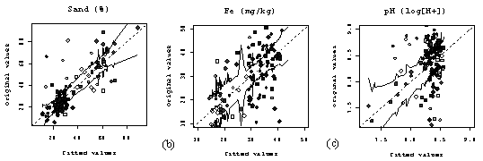
Improving the fuzzy classification using quantitative colour measurements
The transformation of the many spectral curve variables to just three chromaticity coordinates permitted the inclusion of the spectral information expressed in colour format into a fuzzy classification. The fuzzy classification procedure outlined in chapter 1 was repeated. The spectrally derive CIE L a b Hue, Luminance and Chroma coordinates (0-10cm soil layer) replaced the observed Munsell values. In the first classification observed colour data and physical and chemical data were used, and in this the second spectrally derived colour and the same soil data. The membership values for each analysis are plotted in Figure 3. 22 showing how the two classifications correspond to each other exactly.
|
Figure
3. 22.
Correlations between fuzzy class memberships from spectral colour and
laboratory data (y-axis) and only laboratory data (x-axis), with soil
types allocations designated by shade and shape (square=cotton,
triangle=transition, round=red). |
The important feature to note is the much larger range of membership values for the classification using spectrally derived colour. This reflects the improved ability of the classification algorithm to distinguish between similar soils. Figure 3. 23 illustrates the improvement in the ability of the FC algorithm to differentiate and allocate each sample to an appropriate group. The average silhouette width has increased from by 10% from 0.33 to 0.38 (Figure 3. 23b). The differentiation between the Red and Cotton soil samples is more distinct (Figure 3. 23a). This improvement in classification quality is reflected in the correlation between sand and iron content and the fuzzy class memberships (Table 3. 2). |
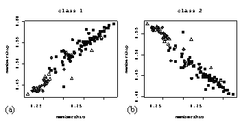
|
The results of stepwise multiple linear regressions between individual wavelengths and soil properties are also presented in Table 3. 2, in order of decreasing strength. The correlations are greater than for the fuzzy memberships, because the regression process is specific to each variable, but results must be interpreted with care. The stepwise MLR procedure required the dataset to split into subgroups to overcome problems of collinearity and singularity when calculating the regression coefficients. The statistical
measures (Aikaike Information Criteria) used to determine the optimal
model and the significant bands are not optimal when there are too many
explanatory variables. These issues are the topic of detailed discussion
in the final chapter and will not be pursued further here. |
Table
3. 2.
Correlations with fuzzy class members and Stepwise-MLR correlation
coefficients between spectra and soil properties. *Indicates significant
at 0.05 level. (Note clay is excluded due to measurement
error). | ||||||||||||||||||||||||||||
|
What is important to note is the strong and significant correlation with sand and iron content and the fuzzy class memberships when spectrally derived colour is used. In contrast no significant correlations were identified between the fuzzy class memberships and the soil properties when observed colour was used in the classification procedure, and therefore regression was not possible. Improving the quality of the colour information by providing quantitatively measured colour data significantly improved the value of the fuzzy classification results at minimal cost. Conclusions
Non-destructive, rapid, cheap and accurate measurement technologies that exploit the interactions of electromagnetic energy with materials at the Earths’ surface are going to be increasingly used to provide increasingly large amounts of diverse environmental data. The dimensionality of hyperspectral data raises several issues during analysis. The results presented in this chapter suggest that reducing the data dimension to a lower spectral resolution typical of hyperspectral imaging devices by convolution does not reduce information content of the data. Principal components is useful for data reduction and facilitated the interpretation of the effects of soil properties on the spectral reflectance curves and provided image variables that were more highly correlated with in-situ variables than the raw image bands. |
Figure
3. 23.
Clusterplots and silhouette plots for two fuzzy classifications performed
using (a + b) selected chemical and physical analyses and
observed soil colour, and (c + d) the same data with spectrally
derived soil colour. | ||||||||||||||||||||||||||||
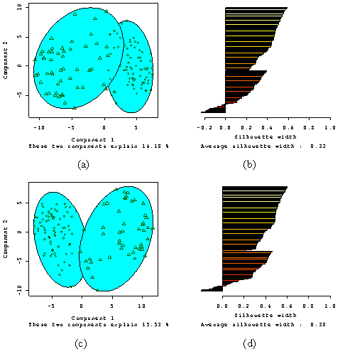
The first three
components contained over 90 % of the data variance. Higher order PCs could
be discarded, without a significant loss of information. The principal
components of the laboratory spectra could be interpreted with reference to
standard texts on reflectance spectroscopy (Clark & Roush, 1984) and soil
spectral reflectance curves (Stoner & Baumgardner, 1981) and more recent
papers using laboratory spectroscopy and hyperspectral remote sensing to
discriminate between soils and predict soil properties (Palacios-Orueta &
Ustin, 1996 and 1998). The principal components exaggerated the features of
interest, the wavelengths that summarised much of the variation in the dataset.
The findings presented in this chapter reflected common observations.
Differences caused by sand and iron content permitted differentiation between
the two major soil types of the region, the Cotton and the Red soil. The
controlling effect that these two properties have on soil colour, and therefore
the spectral measurements masked the effects of other soil properties that
varied less such as organic matter, yet which commonly exert a strong influence
on spectral reflectance.
There exist many ways to express
colour, as many individual measurements at individual wavelengths or as
trivariate colour coordinates. The latter are an invaluable means of reducing
the dimensionality of reflectance measurements, whilst providing variables that
can be clearly understood, and with which soil experts have long been familiar.
In contrast to the factors calculated by a principal components analysis, which
must be interpreted uniquely for each dataset and study area, colour coordinates
have a unique and universal meaning and physical
interpretation.
Transforming spectra into colour
provides a means of ‘bridging the gap’ between traditional and modern colour
measurement techniques, of providing data in a similar format, that permitted
direct comparison of vision matched and machine measured colour. This enabled a
verification of the physical basis of the colour matching process. Evidently,
changing illumination conditions when in the field and various complex and
incompletely understood human vision effects cause the distribution of values
that are assigned to be wider than those that are provided by measurement.
Nevertheless, the allocation of samples to modal soil types, done primarily on
the basis of colour matches made in the field, effectively repartitioned samples
into groups having strong within group similarity of chemical and physical
properties and significant differences between groups. This allocation proved to
be the same as that provided using quantitative and therefore more reliable
colour data. There are strong and meaningful relationships between observed and
spectrally derived colour, when expressed in a common format. This is important
because the former are qualitative and subject to human error and bias and
therefore require validation. Colour observations made in the field can be used
as a diagnostic criteria to classify the soil and to predict average values and
variances for selected properties that strongly affect soil colour, in this
instance iron content or soil texture.
Knowledge of the soil colour by itself is of interest, but at present of little use. Colour is however correlated with soil properties that reflect and condition soil processes, formation and therefore potential use. As a cheap-to-measure variable colour has long been used as a surrogate for direct measurements. Several different colour systems can be used to define colours. These results show that the correlations between soil properties and the Munsell code are stronger than those between the same properties and colour coordinates that do not share the same underlying perceptual basis, of Hue, Value and Chroma such as the CIE Y xyz, XYZ, CIE L*a*b* and rgb colour spaces. The process of transformation did not itself introduce any uncertainty, they are exact transformations and the CIE L*a*b* representation was the last to be calculated in a long chain of processing steps. If transformation reduced correlation by the introduction of error, then this representation should have shown the weakest correlations. Nevertheless on average the modelled relationships were weak and possible only for the controlling soil variables, texture and iron content, despite the indication that soil colour provides reliable information as to the likely distribution of pH, ECe and organic matter content, indirectly via a soil pedon type assignment.
These results highlight the
important fact that the possible uses of data and reliability with which
information can be derived from data, are defined at the outset by the quality
of the measurement procedure. The human eye‑brain combination is able to
perceive subtleties with acuity beyond that which we can express in words and
individuals perceive colours differently. This leads to error and disagreement
(Post, 1993). Qualitative measurement places a ceiling on the reliability of
estimates. If this situation is to change then soil colour measurements must be
made quantitatively in the field, using hand-held spectrometers, tristimulus and
trichromaticity meters. These instruments offer the possibility to provide
accurate colour measurements in any of the coordinate systems. The challenge to
be overcome, related to their use in the field, would be to control illumination
and soil sample conditions. In this study the data was simulated from precise
reflectance measurements made on crushed and sieved (<2mm) soil. There is
considerable evidence to suggest that soil aggregation and variable moisture
content would introduce greater variability to the measurements. It remains to
be tested whether this would significantly reduce the quality of the data for
inclusion in models for the prediction of soil
properties.
It remains to investigate the spatial information contained in the spectral data and to investigate ways to use the individual wavelength measurements most effectively in regression models for soil properties. The second of these questions will form the focus of the final chapter of this thesis, after the colour representation of spectral data has been investigated further for spatial information content. Quantitative measurements of soil colour provide a more precise and continuous description of soil colour that corresponds to our understanding of soil as a continuous phenomenon. The intuitive representational nature of colour data should provide a useful synthetic summary of spatial variation. Colour data, in any of the formats described above can be kriged to generate spatial predictions. Consideration of the representational qualities of each colour space in light of the mapping objectives should determine which system is used. Each colour space has specific numerical properties that should influence the choice of interpolation method. These subjects are the focus of the next chapter.